![]()
Note: This guidebook for the TI-84 Plus or TI-84 Plus Silver Edition with operating system (OS) version 2.55MP. If your calculator has a previous OS version, your screens may look different and some features may not be available. You can download the latest OS education.ti.com/guides.
Texas Instruments makes no warranty, either express or implied, including but not limited to any implied warranties of merchantability and fitness for a particular purpose, regarding any programs or book materials and makes such materials available solely on an "as-is" basis. In no event shall Texas Instruments be liable to anyone for special, collateral, incidental, or consequential damages in connection with or arising out of the purchase or use of these materials, and the sole and exclusive liability of Texas Instruments, regardless of the form of action, shall not exceed the purchase price of this product. Moreover, Texas Instruments shall not be liable for any claim of any kind whatsoever against the use of these materials by any other party.
© 2004–2010 Texas Instruments Incorporated
Vernier EasyData, Vernier LabPro, and Vernier Go! Motion are a trademarks of Vernier Software & Technology.
Important Information ii
Chapter 1:
Operating the TI-84 Plus Silver Edition 1
Documentation Conventions 1
TI-84 Plus Keyboard 1
Turning On and Turning Off the TI-84 Plus 3
Setting the Display Contrast 4
The Display 5
Interchangeable Faceplates 8
Using the Clock 9
Entering Expressions and Instructions 11
Setting Modes 14
Using TI-84 Plus Variable Names 19
Storing Variable Values 20
Recalling Variable Values 21
Scrolling Through Previous Entries on the Home Screen 22
ENTRY (Last Entry) Storage Area 22
TI-84 Plus Menus 25
VARS and VARS Y-VARS Menus 27
Equation Operating System (EOSâ„¢) 29
Special Features of the TI-84 Plus 30
Other TI-84 Plus Features 31
Error Conditions 33
Chapter 2:
Math, Angle, and Test Operations 35
Getting Started: Coin Flip 35
Keyboard Math Operations 36
MATH Operations 38
Using the Equation Solver 42
MATH NUM (Number) Operations 45
Entering and Using Complex Numbers 50
MATH CPX (Complex) Operations 54
MATH PRB (Probability) Operations 56
ANGLE Operations 59
TEST (Relational) Operations 62
TEST LOGIC (Boolean) Operations 63
Chapter 3:
Function Graphing 65
Getting Started: Graphing a Circle 65
Defining Graphs 66
Setting the Graph Modes 67
Defining Functions 68
Selecting and Deselecting Functions 69
Setting Graph Styles for Functions 71
Setting the Viewing Window Variables 73
Setting the Graph Format 74
Displaying Graphs 76
Exploring Graphs with the Free-Moving Cursor 78
Exploring Graphs with TRACE 78
Exploring Graphs with the ZOOM Instructions 80
Using ZOOM MEMORY 85
Using the CALC (Calculate) Operations 87
Chapter 4:
Parametric Graphing 91
Getting Started: Path of a Ball 91
Defining and Displaying Parametric Graphs 93
Exploring Parametric Graphs 95
Chapter 5:
Polar Graphing 97
Getting Started: Polar Rose 97
Defining and Displaying Polar Graphs 98
Exploring Polar Graphs 100
Chapter 6:
Sequence Graphing 102
Getting Started: Forest and Trees 102
Defining and Displaying Sequence Graphs 103
Selecting Axes Combinations 107
Exploring Sequence Graphs 107
Graphing Web Plots 109
Using Web Plots to Illustrate Convergence 110
Graphing Phase Plots 111
Comparing TI-84 Plus and TI-82 Sequence Variables 113
Keystroke Differences Between TI-84 Plus
and TI-82 114
Chapter 7:
Tables 115
Getting Started: Roots of a Function 115
Setting Up the Table 116
Defining the Dependent Variables 117
Displaying the Table 118
Chapter 8:
Draw Instructions 121
Getting Started: Drawing a Tangent Line 121
Using the DRAW Menu 122
Clearing Drawings 123
Drawing Line Segments 124
Drawing Horizontal and Vertical Lines 125
Drawing Tangent Lines 126
Drawing Functions and Inverses 127
Shading Areas on a Graph 128
Drawing Circles 128
Placing Text on a Graph 129
Using Pen to Draw on a Graph 130
Drawing Points on a Graph 131
Drawing Pixels 132
Storing Graph Pictures (Pic) 134
Recalling Graph Pictures (Pic) 135
Storing Graph Databases (GDB) 135
Recalling Graph Databases (GDB) 136
Chapter 9:
Split Screen 137
Getting Started: Exploring the Unit Circle 137
Using Split Screen 138
Horiz (Horizontal) Split Screen 139
G-T (Graph-Table) Split Screen 140
TI-84 Plus Pixels in Horiz and G-T Modes 141
Chapter 10:
Matrices 143
Getting Started: Using the MTRX Shortcut Menu 143
Getting Started: Systems of Linear Equations 144
Defining a Matrix 145
Viewing and Editing Matrix Elements 146
Using Matrices with Expressions 148
Displaying and Copying Matrices 149
Using Math Functions with Matrices 151
Using the MATRX MATH Operations 154
Chapter 11:
Lists 161
Getting Started: Generating a Sequence 161
Naming Lists 162
Storing and Displaying Lists 163
Entering List Names 164
Attaching Formulas to List Names 165
Using Lists in Expressions 167
LIST OPS Menu 168
LIST MATH Menu 175
Chapter 12:
Statistics 178
Getting Started: Pendulum Lengths and Periods 178
Setting Up Statistical Analyses 184
Using the Stat List Editor 185
Attaching Formulas to List Names 188
Detaching Formulas from List Names 190
Switching Stat List Editor Contexts 190
Stat List Editor Contexts 192
STAT EDIT Menu 193
Regression Model Features 195
STAT CALC Menu 198
Statistical Variables 206
Statistical Analysis in a Program 207
Statistical Plotting 208
Statistical Plotting in a Program 212
Chapter 13:
Inferential Statistics and Distributions 215
Getting Started: Mean Height of a Population 215
Inferential Stat Editors 218
STAT TESTS Menu 221
Inferential Statistics Input Descriptions 239
Test and Interval Output Variables 240
Distribution Functions 241
Distribution Shading 248
Chapter 14:
Applications 251
The Applications Menu 251
Getting Started: Financing a Car 252
Getting Started: Computing Compound Interest 253
Using the TVM Solver 253
Using the Financial Functions 254
Calculating Time Value of Money (TVM) 255
Calculating Cash Flows 257
Calculating Amortization 258
Calculating Interest Conversion 261
Finding Days between Dates/Defining Payment Method 261
Using the TVM Variables 262
The EasyDataâ„¢ Application 263
Chapter 15:
CATALOG, Strings, Hyperbolic Functions 266
Browsing the TI-84 Plus CATALOG 266
Entering and Using Strings 267
Storing Strings to String Variables 268
String Functions and Instructions in the CATALOG 269
Hyperbolic Functions in the CATALOG 273
Chapter 16:
Programming 275
Getting Started: Volume of a Cylinder 275
Creating and Deleting Programs 276
Entering Command Lines and Executing Programs 278
Editing Programs 279
Copying and Renaming Programs 280
PRGM CTL (Control) Instructions 281
PRGM I/O (Input/Output) Instructions 288
Calling Other Programs as Subroutines 293
Running an Assembly Language Program 294
Chapter 17:
Activities 296
The Quadratic Formula 296
Box with Lid 299
Comparing Test Results Using Box Plots 306
Graphing Piecewise Functions 308
Graphing Inequalities 309
Solving a System of Nonlinear Equations 310
Using a Program to Create the Sierpinski Triangle 311
Graphing Cobweb Attractors 312
Using a Program to Guess the Coefficients 313
Graphing the Unit Circle and Trigonometric Curves 315
Finding the Area between Curves 316
Using Parametric Equations: Ferris Wheel Problem 317
Demonstrating the Fundamental Theorem of Calculus 319
Computing Areas of Regular N-Sided Polygons 321
Computing and Graphing Mortgage Payments 323
Chapter 18:
Memory and Variable Management 326
Checking Available Memory 326
Deleting Items from Memory 329
Clearing Entries and List Elements 329
Archiving and UnArchiving Variables 330
Resetting the TI-84 Plus 333
Grouping and Ungrouping Variables 336
Garbage Collection 339
ERR:ARCHIVE FULL Message 343
Chapter 19:
Communication Link 344
Getting Started: Sending Variables 344
TI-84 Plus LINK 345
Selecting Items to Send 347
Receiving Items 350
Backing Up RAM Memory 351
Error Conditions 352
Appendix A:
Functions and Instructions 354
Appendix B:
Reference Information 383
Variables 383
Statistics Formulas 384
Financial Formulas 387
Important Things You Need to Know About Your TI-84 Plus 391
Error Conditions 394
Accuracy Information 398
Appendix C:
Service and Warranty Information 400
Texas Instruments Support and Service 400
Battery Information 400
In Case of Difficulty 402
In the body of this guidebook, TI-84 Plus refers to the TI-84 Plus Silver Edition, but all of the instructions, examples, and functions in this guidebook also work for the TI-84 Plus. The two graphing calculators differ only in available RAM memory, interchangeable faceplates, and Flash application ROM memory. Sometimes, as in Chapter 19, the full name TI-84 Plus Silver Edition is used to distinguish it from the TI-84 Plus.
A new MODE menu item, STAT WIZARDS is available with OS version 2.55MP for syntax entry help for commands and functions in the STAT CALC menu, DISTR DISTR menu, DISTR DRAW menu and the seq( function (sequence) in the LIST OPS menu. When selecting a supported statistics command, regression or distribution with the STAT WIZARDS setting ON: (the default setting) a syntax help (wizard) screen is displayed. The wizard allows the entry of required and optional arguments. The function or command will paste with the entered arguments to the Home Screen history or in most other locations where the cursor is available for input. If a command or function is accessed from [CATALOG] the command or function will paste without wizard support. Run the Catalog Help application ([APPS]) for more syntax help when needed.
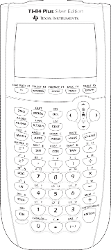
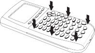
Generally, the keyboard is divided into these zones: graphing keys, editing keys, advanced function keys, and scientific calculator keys.
Keyboard Zones
Graphing — Graphing keys access the interactive graphing features. The third function of these keys ([ALPHA] [F1] [F4]) displays the shortcut menus, which include templates for fractions, n/d, quick matrix entry, and some of the functions found on the MATH and VARS menus.
Editing — Editing keys allow you to edit expressions and values.
Advanced — Advanced function keys display menus that access the advanced functions.
Scientific — Scientific calculator keys access the capabilities of a standard scientific calculator.
TI-84 Plus Silver Edition
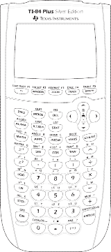
Graphing Keys are in the top row. Editing Keys are in the second and third rows.
Advanced Function Keys are in the fourth row.
Scientific Calculator Keys are in rows five through ten.
Using the Color-Coded Keyboard
The keys on the TI-84 Plus are color-coded to help you easily locate the key you need.
The light colored keys are the number keys. The keys along the right side of the keyboard are the common math functions. The keys across the top set up and display graphs. The [APPS] key provides access to applications such as the Inequality Graphing, Transformation Graphing, Conic Graphing, Polynomial Root Finder and Simultaneous Equation Solver, and Catalog Help.
The primary function of each key is printed on the keys. For example, when you press [MATH], the
MATH menu is displayed.
Using the [2nd] and [ALPHA] Keys
The secondary function of each key is printed above the key. When you press the [2nd] key, the character, abbreviation, or word printed above the other keys becomes active for the next keystroke. For example, when you press [2nd] and then [MATH], the TEST menu is displayed. This guidebook describes this keystroke combination as [2nd] [TEST].
Many keys also have a third function. These functions are printed above the keys in the same color as the [ALPHA] key. The third functions enter alphabetic characters and special symbols as well as access SOLVE and shortcut menus. For example, when you press [ALPHA] and then [MATH], the letter A is entered. This guidebook describes this keystroke combination as [ALPHA] [A].
If you want to enter several alphabetic characters in a row, you can press [2nd] [A-LOCK] to lock the alpha key in the On position and avoid having to press [ALPHA] multiple times. Press [ALPHA] a second time to unlock it.
Note: The flashing cursor changes to Reverse A when you press [ALPHA], even if you are accessing a function or a menu.
Second row, first key is [2nd]
Accesses the second function printed above each key.
Third row, first key is [ALPHA]
Accesses the third function printed above each key.
[ALPHA] and top row keys one through four [F1]-[F4] Access shortcut menus for functionality including templates for fractions, n/d, and other functions.
To turn on the TI-84 Plus, press [ON]. An information screen displays reminding you that you can press [ALPHA] [F1] - [F4] to display the shortcut menus. This message also displays when you reset RAM.
ï‚„ To continue but not see this information screen again, press 1.
ï‚„ To continue and see this information screen again the next time you turn on the TI-84 Plus, press 2.
If you previously had turned off the graphing calculator by pressing [2nd] [OFF], the TI-84 Plus displays the home screen as it was when you last used it and clears any error. (The information screen displays first, unless you chose not to see it again.) If the home screen is blank, press [up key] to scroll through the history of previous calculations.
If Automatic Power Downâ„¢ (APDâ„¢) had previously turned off the graphing calculator, the TI-84 Plus will return exactly as you left it, including the display, cursor, and any error.
If the TI-84 Plus is turned off and connected to another graphing calculator or personal computer, any communication activity will “wake up†the TI-84 Plus.
To prolong the life of the batteries, APDâ„¢ turns off the TI-84 Plus automatically after about five minutes without any activity.
Turning Off the Graphing Calculator
To turn off the TI-84 Plus manually, press [2nd] [OFF].
All settings and memory contents are retained by the Constant Memoryâ„¢ function.
Any error condition is cleared.
Batteries
The TI-84 Plus uses five batteries: four AAA alkaline batteries and one button cell backup battery. The backup battery provides auxiliary power to retain memory while you replace the AAA batteries. To replace batteries without losing any information stored in memory, follow the steps in Appendix C.
Adjusting the Display Contrast
You can adjust the display contrast to suit your viewing angle and lighting conditions. As you change the contrast setting, a number from 0 (lightest) to 9 (darkest) in the top-right corner indicates the current level. You may not be able to see the number if contrast is too light or too dark.
Note: The TI-84 Plus has 40 contrast settings, so each number 0 through 9 represents four settings.
The TI-84 Plus retains the contrast setting in memory when it is turned off. To adjust the contrast, follow these steps.
ï‚„ Press [2nd] [up key] to darken the screen one level at a time.
ï‚„ Press [2nd] [down key] to lighten the screen one level at a time.
Note: If you adjust the contrast setting to 0, the display may become completely blank. To restore the screen, press [2nd] [up key] until the display reappears.
When to Replace Batteries
When the batteries are low, a low-battery message is displayed when you turn on the graphing calculator.
To replace the batteries without losing any information in memory, follow the steps in Appendix C.
Generally, the graphing calculator will continue to operate for one or two weeks after the low- battery message is first displayed. After this period, the TI-84 Plus will turn off automatically and the unit will not operate. Batteries must be replaced. All memory should be retained.
Note:
The operating period following the first low-battery message could be longer than two weeks if you use the graphing calculator infrequently.
Always replace batteries before attempting to install a new operating system.
Types of Displays
The TI-84 Plus displays both text and graphs. Chapter 3 describes graphs. Chapter 9 describes how the TI-84 Plus can display a horizontally or vertically split screen to show graphs and text simultaneously.
Home Screen
The home screen is the primary screen of the TI-84 Plus. On this screen, enter instructions to execute and expressions to evaluate. The answers are displayed on the same screen. Most calculations are stored in the history on the home screen. You can press [up key] and [down key] to scroll through the history of entries on the home screen and you can paste the entries or answers to the current entry line.
Displaying Entries and Answers
When text is displayed, the TI-84 Plus screen can display a maximum of 8 lines with a maximum of 16 characters per line in Classic mode. In MathPrintâ„¢ mode, fewer lines and fewer characters per line may be displayed.
If all lines of the display are full, text scrolls off the top of the display.
To view previous entries and answers, press [up key].
To copy a previous entry or answer and paste it to the current entry line, move the cursor to the entry or answer you want to copy and press [ENTER].
Note: List and matrix outputs cannot be copied. If you try to copy and paste a list or matrix output, the cursor returns to the input line.
If an expression on the home screen, the Y= editor (Chapter 3), or the program editor (Chapter 16) is longer than one line, it wraps to the beginning of the next line in Classic mode. In MathPrintâ„¢ mode, an expression on the home screen or Y= editor that is longer than one line scrolls off the screen to the right. An arrow on the right side of the screen indicates that you can scroll right to see more of the expression. In numeric editors such as the window screen (Chapter 3), a long expression scrolls to the right and left in both Classic and MathPrintâ„¢ modes. Press [2nd] [right key] to move the cursor to the end of the line. Press [2nd] [left key] to move the cursor to the beginning of the line.
When an entry is executed on the home screen, the answer is displayed on the right side of the next line.
![]()
The entry is displayed first.
The answer is displayed on the right side of the next line.
The mode settings control the way the TI-84 Plus interprets expressions and displays answers.
If an answer, such as a list or matrix, is too long to display entirely on one line, an arrow (MathPrintâ„¢) or an ellipsis (Classic) is displayed to the right or left. Press [right key] and [left key] to display the answer.
MathPrintâ„¢ Classic
![]()
Entry above, ![]() answer below
answer below
![]()
![]()
Using Shortcut Menus
[ALPHA] and first key of top row [F1] Opens FRAC menu. [ALPHA] and second key of top row [F2] Opens FUNC menu. [ALPHA] and third key of top row [F3] Opens MTRX menu. [ALPHA] and fourth key of top row [F4] Opens YVAR menu.
Shortcut menus allow quick access to the following:
Templates to enter fractions and selected functions from the MATH MATH and MATH NUM menus as you would see them in a textbook. Functions include absolute value, summation, numeric differentiation, numeric integration, and log base n.
Matrix entry.
Names of function variables from the VARS Y-VARS menu.
Initially, the menus are hidden. To open a menu, press [ALPHA] plus the F-key that corresponds to the menu, that is, [F1] for FRAC, [F2] for FUNC, [F3] for MTRX, or [F4] for YVAR. To select a menu item, either press the number corresponding to the item, or use the arrow keys to move the cursor to the appropriate line and then press [ENTER].
All shortcut menu items except matrix templates can also be selected using standard menus. For example, you can choose the summation template from three places:
FUNC shortcut menu  MATH MATH menu
  Catalog
The shortcut menus are available to use where input is allowed. If the calculator is in Classic mode, or if a screen is displayed that does not support MathPrintâ„¢ display, entries will be displayed in Classic display. The MTRX menu is only available in MathPrintâ„¢ mode on the home screen and in the Y = editor.
Note: Shortcut menus may not be available if [ALPHA] plus F-key combinations are used by an application that is running, such as Inequality Graphing or Transformation Graphing.
Returning to the Home Screen
To return to the home screen from any other screen, press [2nd] [QUIT].
Busy Indicator
When the TI-84 Plus is calculating or graphing, a vertical moving line is displayed as a busy indicator in the top-right corner of the screen. When you pause a graph or a program, the busy indicator becomes a vertical moving dotted line.
Display Cursors
In most cases, the appearance of the cursor indicates what will happen when you press the next key or select the next menu item to be pasted as a character.
![]()
![]()
Cursor Appearance Effect of Next Keystroke
Entry Solid rectangle
![]()
Insert Underline
![]()
![]()
Second Reverse arrow Reverse upward arrow
![]()
Alpha Reverse A
A
![]()
Full Checkerboard rectangle
â–
A character is entered at the cursor; any existing character is overwritten
A character is inserted in front of the cursor location
A 2nd character is entered or a 2nd operation is executed
An alpha character is entered, SOLVE is executed, or shortcut menus are displayed.
No entry; the maximum characters are entered at a prompt or memory is full
![]()
MathPrintâ„¢ Right arrow The cursor moves to either the next part of the
![]() template or out of the template.
template or out of the template.
![]()
If you press [ALPHA] during an insertion, the cursor becomes an underlined A (A). If you press [2nd]
during an insertion, the underlined cursors becomes an underlined upward arrow.
Note: If you highlight a small character such as a colon or a comma and then press [ALPHA] or
[2nd], the cursor does not change because the cursor width is too narrow.
Graphs and editors sometimes display additional cursors, which are described in other chapters.
The TI-84 Plus Silver Edition has interchangeable faceplates that let you customize the appearance of your unit. To purchase additional faceplates, refer to the TI Online Store at education.ti.com.
Removing a Faceplate

Lift the tab at the bottom edge of the faceplate away from the TI-84 Plus Silver Edition case.
Carefully lift the faceplate away from the unit until it releases. Be careful not to damage the faceplate or the keyboard.
Installing New Faceplates
Align the top of the faceplate in the corresponding grooves of the TI-84 Plus Silver Edition case.
Gently click the faceplate into place. Do not force.
Make sure you gently press each of the grooves to ensure the faceplate is installed properly. See the diagram for proper groove placement.
Use the clock to set the time and date, select the clock display format, and turn the clock on and off. The clock is turned on by default and is accessed from the mode screen.
Displaying the Clock Settings
Press [MODE].
Press the [down key] to move the cursor to
SET CLOCK.
Press [ENTER].
Changing the Clock Settings
Press the [right key] or [left key] to highlight the date format you want. Press [ENTER].
Press [down key] to highlight YEAR. Press
[CLEAR] and type the year.
Press [down key] to highlight MONTH. Press
[CLEAR] and type the number of the month (1-12).
Press [down key] to highlight DAY. Press [CLEAR]
and type the date.
Press [down key] to highlight TIME. Press [right key] or [left key] to highlight the time format you want. Press [ENTER].
Press [down key] to highlight HOUR. Press [CLEAR] and type the hour (a number from 1-12 or 0-23).
Press [down key] to highlight MINUTE. Press [CLEAR] and type the minutes (a number from 0-59).
Press [down key] to highlight AM/PM. Press [right key] or [left key] to highlight the format. Press [ENTER].
To save changes, press [down key] to highlight
SAVE. Press [ENTER].
Error Messages
If you type the wrong date for the month, for example, June 31 (June does not have 31 days), you will receive an error message with two choices:
To quit the clock application and return to the home screen, select 1: Quit.
— or —
To return to the clock application and correct the error, select 2: Goto.
Turning the Clock On
There are two options to turn the clock on. One option is through the MODE screen, the other is through the Catalog.
Using the Mode Screen to turn the clock on
If the clock is turned off, Press [down key] to highlight TURN CLOCK ON.
Press [ENTER] [ENTER].
Using the Catalog to turn the clock on
If the clock is turned off, Press [2nd] [CATALOG]
Press [down key] or [up key] to scroll the CATALOG
until the selection cursor points to ClockOn.
Press [ENTER] [ENTER].
Turning the Clock Off
Press [2nd] [CATALOG].
Press [down key] or [up key] to scroll the CATALOG
until the selection cursor points to ClockOff.
Press [ENTER] [ENTER].
What Is an Expression?
An expression is a group of numbers, variables, functions and their arguments, or a combination of these elements. An expression evaluates to a single answer. On the TI-84 Plus, you enter an expression in the same order as you would write it on paper. For example, pi Rsquared is an expression.
![]()
You can use an expression on the home screen to calculate an answer. In most places where a value is required, you can use an expression to enter a value.
Entering an Expression
To create an expression, you enter numbers, variables, and functions using the keyboard and menus. An expression is completed when you press [ENTER], regardless of the cursor location. The entire expression is evaluated according to Equation Operating System (EOSâ„¢) rules, and the answer is displayed according to the mode setting for Answer.
Most TI-84 Plus functions and operations are symbols comprising several characters. You must enter the symbol from the keyboard or a menu; do not spell it out. For example, to calculate the log of 45, you must press [LOG] 45. Do not enter the letters L, O, and G. If you enter L O G, the
TI-84 Plus interprets the entry as implied multiplication of the variables L, O, and G.
Calculate 3.76 divided by (negative 7.9 + square root of 5) + 2 log 45.
3 [decimal point] 76 [division key] [open paren] [open paren negative close paren] 7 [decimal point]
9 [addition key]
[2nd] [square root key]5 [close paren] [close paren] [addition key] 2 [LOG] 45 [close paren][ENTER]
![]()
![]()
MathPrintâ„¢ Classic
Multiple Entries on a Line
To enter two or more expressions or instructions on a line, separate them with colons ([ALPHA] [:]). All instructions are stored together in last entry (ENTRY).
![]()
Entering a Number in Scientific Notation
Enter the part of the number that precedes the exponent. This value can be an expression.
Press [2nd] [EE]. E is pasted to the cursor location.
Enter the exponent, which can be one or two digits.
Note: If the exponent is negative, press [open paren negative close paren], and then enter the exponent.
![]()
When you enter a number in scientific notation, the TI-84 Plus does not automatically display answers in scientific or engineering notation. The mode settings and the size of the number determine the display format.
Functions
A function returns a value. For example, division, subtraction, addition, square root, and log( are the functions in the example on the previous page. In general, the first letter of each function is lowercase on the TI-84 Plus. Most functions take at least one argument, as indicated by an open parenthesis following the name. For example, sin( requires one argument, sin(value).
Note: The Catalog Help App contains syntax information for most of the functions in the catalog.
Instructions
An instruction initiates an action. For example, ClrDraw is an instruction that clears any drawn elements from a graph. Instructions cannot be used in expressions. In general, the first letter of each instruction name is uppercase. Some instructions take more than one argument, as indicated by an open parenthesis at the end of the name. For example, Circle( requires three arguments, Circle(X, Y, radius).
Interrupting a Calculation
To interrupt a calculation or graph in progress, which is indicated by the busy indicator, press [ON]. When you interrupt a calculation, a menu is displayed.
To return to the home screen, select 1:Quit.
To go to the location of the interruption, select 2:Goto. When you interrupt a graph, a partial graph is displayed.
To return to the home screen, press [CLEAR] or any non-graphing key.
To restart graphing, press a graphing key or select a graphing instruction.
TI-84 Plus Edit Keys
![]()
Keystrokes Result
![]()
[right key] or [left key] Moves the cursor within an expression; these keys repeat.
![]()
[up key] or [down key] Moves the cursor from line to line within an expression that occupies more than one line; these keys repeat.
Moves the cursor from term to term within an expression in MathPrintâ„¢ mode; these keys repeat.
On the home screen, scrolls through the history of entries and answers.
![]()
[2nd] [left key] Moves the cursor to the beginning of an expression.
![]()
[2nd] [right key] Moves the cursor to the end of an expression.
![]()
[2nd] [up key] On the home screen, moves the cursor out of a MathPrintâ„¢ expression.
In the Y=editor, moves the cursor from a MathPrintâ„¢ expression to the previous
Y-var.
![]()
[2nd] [down key] In the Y=editor, moves the cursor from a MathPrint â„¢ expression to the next Y- var.
![]()
[ENTER] Evaluates an expression or executes an instruction.
![]()
[CLEAR] On a line with text on the home screen, clears the current line.
On a blank line on the home screen, clears everything on the home screen.
In an editor, clears the expression or value where the cursor is located; it does not store a zero.
![]()
![]()
Keystrokes Result
![]()
[DEL] Deletes a character at the cursor; this key repeats.
![]()
[2nd] [INS] Changes the cursor to an underline ( ); inserts characters in front of the underline cursor; to end insertion, press [2nd] [INS] or press [left key], [up key], [right key], or [down key].
![]()
[2nd] Changes the cursor to reverse upward arrow; the next keystroke performs a 2nd function (displayed above a key and to the left); to cancel 2nd, press [2nd] again.
![]()
[ALPHA] Changes the cursor to reverse A; the next keystroke performs a third function of that key (displayed above a key and to the right), executes SOLVE (Chapters 10 and 11), or accesses a shortcut menu; to cancel [ALPHA], press [ALPHA] or press [left key], [up key], [right key], or [down key].
![]()
[2nd] [A-LOCK] Changes the cursor to reverse A; sets alpha-lock; subsequent keystrokes access the third functions of the keys pressed; to cancel alpha-lock, press [ALPHA]. If you are prompted to enter a name such as for a group or a program, alpha-lock is set automatically.
![]()
[X,T, theta, n] Pastes an X in Func mode, a T in Par mode, a theta in Pol mode, or an n in Seq
mode with one keystroke.
![]()
Checking Mode Settings
Mode settings control how the TI-84 Plus displays and interprets numbers and graphs. Mode settings are retained by the Constant ‘Memory™ feature when the TI-84 Plus is turned off. All numbers, including elements of matrices and lists, are displayed according to the current mode settings.
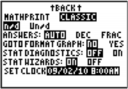
To display the mode settings, press [MODE]. The current settings are highlighted. Defaults are highlighted below. The following pages describe the mode settings in detail.
![]()
Normal Sci Eng Numeric notation
Float 0123456789 Number of decimal places in answers
Radian Degree Unit of angle measure
Func Par Pol Seq Type of graphing
Connected Dot Whether to connect graph points
Sequential Simul Whether to plot simultaneously
Real a+bi re^theta i Real, rectangular complex, or polar complex
Full Horiz G-T Full screen, two split-screen modes
MathPrint Classic Controls whether inputs and outputs on the home screen and in
the Y= editor are displayed as they are in textbooks
n/d Un/d Displays results as simple fractions or mixed fractions
Answers: Auto Dec Frac Controls the format of the answers
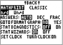
![]()
![]()
GoTo Format Graph: No Yes Shortcut to the Format Graph screen ([2nd] [FORMAT])
StatDiagnostics: Off On Determines which information is displayed in a statistical
regression calculation
StatWizards: On Off Determines if syntax help prompts are provided for optional and
required arguments for many statistical, regression and
distribution commands and functions.
On: Selection of menu items in STAT CALC, DISTR DISTR, DISTR DRAW and seq( in LIST OPS displays a screen which provides syntax help (wizard) for the entry of required and optional arguments into the command or function. The function or command will paste the entered arguments to the Home Screen history or to most other locations where the cursor is available for input. Some calculations will compute directly from the wizard. If a command or function is accessed from [CATALOG] the command or function will paste without wizard support. Run the Catalog Help application ([APPS]) for more syntax help when needed.
Off: The function or command will paste to the cursor location with no syntax help (wizard).
Set Clock Sets the time and date
![]()
Changing Mode Settings
To change mode settings, follow these steps.
Press [down key] or [up key] to move the cursor to the line of the setting that you want to change.
Press [right key] or [left key] to move the cursor to the setting you want.
Press [ENTER].
Setting a Mode from a Program
You can set a mode from a program by entering the name of the mode as an instruction; for example, Func or Float. From a blank program command line, select the mode setting from the mode screen; the instruction is pasted to the cursor location.
![]()
Normal, Sci, Eng
Notation modes only affect the way an answer is displayed on the home screen. Numeric answers can be displayed with up to 10 digits and a two-digit exponent and as fractions. You can enter a number in any format.
Normal notation mode is the usual way we express numbers, with digits to the left and right of the decimal, as in 12345.67.
Sci (scientific) notation mode expresses numbers in two parts. The significant digits display with one digit to the left of the decimal. The appropriate power of 10 displays to the right of E, as in 1.234567E4.
Eng (engineering) notation mode is similar to scientific notation. However, the number can have one, two, or three digits before the decimal; and the power-of-10 exponent is a multiple of three, as in 12.34567E3.
Note: If you select Normal notation, but the answer cannot display in 10 digits (or the absolute value is less than .001), the TI-84 Plus expresses the answer in scientific notation.
Float, 0123456789
Float (floating) decimal mode displays up to 10 digits, plus the sign and decimal.
0123456789 (fixed) decimal mode specifies the number of digits (0 through 9) to display to the right of the decimal for decimal answers.
The decimal setting applies to Normal, Sci, and Eng notation modes.
The decimal setting applies to these numbers, with respect to the Answer mode setting:
An answer displayed on the home screen
Coordinates on a graph (Chapters 3, 4, 5, and 6)
The Tangent( DRAW instruction equation of the line, x, and dy/dx values (Chapter 8)
Results of CALCULATE operations (Chapters 3, 4, 5, and 6)
The regression equation stored after the execution of a regression model (Chapter 12)
Radian, Degree
Angle modes control how the TI-84 Plus interprets angle values in trigonometric functions and polar/rectangular conversions.
Radian mode interprets angle values as radians. Answers display in radians.
Degree mode interprets angle values as degrees. Answers display in degrees.
Func, Par, Pol, Seq
Graphing modes define the graphing parameters. Chapters 3, 4, 5, and 6 describe these modes in detail.
Func (function) graphing mode plots functions, where Y is a function of X (Chapter 3).
Par (parametric) graphing mode plots relations, where X and Y are functions of T (Chapter 4).
Pol (polar) graphing mode plots functions, where r is a function of theta (Chapter 5).
Seq (sequence) graphing mode plots sequences (Chapter 6).
Connected, Dot
Connected plotting mode draws a line connecting each point calculated for the selected functions.
Dot plotting mode plots only the calculated points of the selected functions.
Sequential, Simul
Sequential graphing-order mode evaluates and plots one function completely before the next function is evaluated and plotted.
Simul (simultaneous) graphing-order mode evaluates and plots all selected functions for a single value of X and then evaluates and plots them for the next value of X.
Note: Regardless of which graphing mode is selected, the TI-84 Plus will sequentially graph all stat plots before it graphs any functions.
Real, a+bi, re^theta i
Real mode does not display complex results unless complex numbers are entered as input. Two complex modes display complex results.
a+bi (rectangular complex mode) displays complex numbers in the form a+bi.
re^theta i (polar complex mode) displays complex numbers in the form re^theta i.
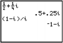
Note: When you use the n/d template,
both n and d must be real numbers. For example, you can enter
![]() (the answer is displayed as a decimal value) but if you enter
(the answer is displayed as a decimal value) but if you enter
![]() ,
a data type error
,
a data type error
displays. To perform division with a complex number in the numerator or denominator, use regular division instead of the n/d template.
Full, Horiz, G-T
Full screen mode uses the entire screen to display a graph or edit screen. Each split-screen mode displays two screens simultaneously.
Horiz (horizontal) mode displays the current graph on the top half of the screen; it displays the home screen or an editor on the bottom half (Chapter 9).
G-T (graph-table) mode displays the current graph on the left half of the screen; it displays the table screen on the right half (Chapter 9).
MathPrintâ„¢, Classic
MathPrintâ„¢ mode displays most inputs and outputs the way they are shown in textbooks, such as
2
1 + 3 and x2dx .
-- --
2 4
1
Classic mode displays expressions and answers as if written on one line, such as 1/2 + 3/4.
Note: If you switch between these modes, most entries will be preserved; however matrix calculations will not be preserved.
n/d, Un/d
n/d displays results as a simple fraction. Fractions may contain a maximum of six digits in the numerator; the value of the denominator may not exceed 9999.
Un/d displays results as a mixed number, if applicable. U, n, and d must be all be integers. If U is a non-integer, the result may be converted U * n/d. If n or d is a non-integer, a syntax error is displayed. The whole number, numerator, and denominator may each contain a maximum of three digits.
Answers: Auto, Dec, Frac
Auto displays answers in a similar format as the input. For example, if a fraction is entered in an expression, the answer will be in fraction form, if possible. If a decimal appears in the expression, the output will be a decimal number.
Dec displays answers as integers or decimal numbers.
Frac displays answers as fractions, if possible.
Note: The Answers mode setting also affects how values in sequences, lists, and tables are displayed. Choose Dec or Frac to ensure that values are displayed in either decimal or fraction form. You can also convert values from decimal to fraction or fraction to decimal using the FRAC shortcut menu or the MATH menu.
GoTo Format Graph: No, Yes
No does not display the FORMAT graph screen, but can always be accessed by pressing
[2nd][FORMAT].
Yes leaves the mode screen and displays the FORMAT graph screen when you press [ENTER] so that you can change the graph format settings. To return to the mode screen, press [MODE].
Stat Diagnostics: Off, On
Off displays a statistical regression calculation without the correlation coefficient (r) or the coefficient of determination (r2).
On displays a statistical regression calculation with the correlation coefficient (r), and the coefficient of determination (r2), as appropriate.
Stat Wizards: On, Off
On: Selection of menu items in STAT CALC, DISTR DISTR, DISTR DRAW and seq( in LIST OPS displays a screen which provides syntax help (wizard) for the entry of required and optional arguments into the command or function. The function or command will paste the entered arguments to the Home Screen history or to most other locations where the cursor is available for input. Some calculations will compute directly from the wizard. If a command or function is accessed from [CATALOG] the command or function will paste without wizard support. Run the Catalog Help application ([APPS]) for more syntax help when needed.
Off: The function or command will paste to the cursor location with no syntax help (wizard)
Set Clock
Use the clock to set the time, date, and clock display formats.
Variables and Defined Items
On the TI-84 Plus you can enter and use several types of data, including real and complex numbers, matrices, lists, functions, stat plots, graph databases, graph pictures, and strings.
The TI-84 Plus uses assigned names for variables and other items saved in memory. For lists, you also can create your own five-character names.
![]()
![]()
Variable Type Names
Real numbers (including fractions)
A, B, ... , Z, theta
![]()
Complex numbers A, B, ... , Z, theta
![]()
Matrices [A], [B], [C], ... , [J]
![]()
Lists L1, L2, L3, L4, L5, L6, and user-defined names
![]()
Functions Y1, Y2, ... , Y9, Y0
![]()
Parametric equations X1T and Y1T, ... , X6T and Y6T
![]()
![]()
Variable Type Names
![]()
Polar functions r1, r2, r3, r4, r5, r6
![]()
Sequence functions u, v, w
![]()
Stat plots Plot1, Plot2, Plot3
![]()
Graph databases GDB1, GDB2, ... , GDB9, GDB0
![]()
Graph pictures Pic1, Pic2, ... , Pic9, Pic0
![]()
Strings Str1, Str2, ... , Str9, Str0
![]()
Apps Applications
![]()
AppVars Application variables
![]()
Groups Grouped variables
![]()
System variables Xmin, Xmax, and others
![]()
Notes about Variables
You can create as many list names as memory will allow (Chapter 11).
Programs have user-defined names and share memory with variables (Chapter 16).
From the home screen or from a program, you can store to matrices (Chapter 10), lists (Chapter 11), strings (Chapter 15), system variables such as Xmax (Chapter 1), TblStart (Chapter 7), and all Y= functions (Chapters 3, 4, 5, and 6).
From an editor, you can store to matrices, lists, and Y= functions (Chapter 3).
From the home screen, a program, or an editor, you can store a value to a matrix element or a list element.
You can use DRAW STO menu items to store and recall graph databases and pictures (Chapter 8).
Although most variables can be archived, system variables including r, T, X, Y, and theta
cannot be archived (Chapter 18)
Apps are independent applications which are stored in Flash ROM. AppVars is a variable holder used to store variables created by independent applications. You cannot edit or change variables in AppVars unless you do so through the application which created them.
Storing Values in a Variable
Values are stored to and recalled from memory using variable names. When an expression containing the name of a variable is evaluated, the value of the variable at that time is used.
To store a value to a variable from the home screen or a program using the [STO right arrow] key, begin on a blank line and follow these steps.
Enter the value you want to store. The value can be an expression.
Press [STO right arrow]. Right arrow is copied to the cursor location.
Press [ALPHA] and then the letter of the variable to which you want to store the value.
Press [ENTER]. If you entered an expression, it is evaluated. The value is stored to the variable.
![]()
Displaying a Variable Value
To display the value of a variable, enter the name on a blank line on the home screen, and then press [ENTER].
![]()
Archiving Variables (Archive, Unarchive)
You can archive data, programs, or other variables in a section of memory called user data archive where they cannot be edited or deleted inadvertently. Archived variables are indicated by asterisks (*) to the left of the variable names. Archived variables cannot be edited or executed. They can only be seen and unarchived. For example, if you archive list L1, you will see that L1 exists in memory but if you select it and paste the name L1 to the home screen, you won’t be able to see its contents or edit it until it is unarchived.
Using Recall (RCL)
To recall and copy variable contents to the current cursor location, follow these steps. To leave
RCL, press [CLEAR].
Press [2nd] [RCL]. RCL and the edit cursor are displayed on the bottom line of the screen.
Enter the name of the variable in one of five ways.
Press [ALPHA] and then the letter of the variable.
Press [2nd] [LIST], and then select the name of the list, or press [2nd] [Ln].
Press [2nd] [MATRIX], and then select the name of the matrix.
Press [VARS] to display the VARS menu or [VARS] [right key] to display the VARS Y-VARS
menu; then select the type and then the name of the variable or function.
Press [ALPHA] [F4] to display the YVAR shortcut menu, then select the name of the function.
Press [PRGM] [left key], and then select the name of the program (in the program editor only).
The variable name you selected is displayed on the bottom line and the cursor disappears.
Press [ENTER]. The variable contents are inserted where the cursor was located before you began these steps.
![]()
Note: You can edit the characters pasted to the expression without affecting the value in memory.
You can scroll up through previous entries and answers on the home screen, even if you have cleared the screen. When you find an entry or answer that you want to use, you can select it and paste it on the current entry line.
Note: List and matrix answers cannot be copied and pasted to the new entry line. However, you can copy the list or matrix command to the new entry line and execute the command again to display the answer.
ï‚„ Press [up key] or [down key] to move the cursor to the entry or answer you want to copy and then press [ENTER]. TThe entry or answer that you copied is automatically pasted on the current input line at the cursor location.
Note: If the cursor is in a MathPrintâ„¢ expression, press [2nd] [up key] to move the cursor out of the expression and then move the cursor to the entry or answer you want to copy.
ï‚„ Press [CLEAR] or [DEL] to delete an entry/answer pair. After an entry/answer pair has been deleted, it cannot be displayed or recalled again.
Using ENTRY (Last Entry)
When you press [ENTER] on the home screen to evaluate an expression or execute an instruction, the expression or instruction is placed in a storage area called ENTRY (last entry). When you turn off the TI-84 Plus, ENTRY is retained in memory.
To recall ENTRY, press [2nd] [ENTRY]. The last entry is pasted to the current cursor location, where you can edit and execute it. On the home screen or in an editor, the current line is cleared and the last entry is pasted to the line.
Because the TI-84 Plus updates ENTRY only when you press [ENTER], you can recall the previous entry even if you have begun to enter the next expression.
![]()
5 [addition key] 7
[ENTER] [2nd] [ENTRY]
Accessing a Previous Entry
The TI-84 Plus retains as many previous entries as possible in ENTRY, up to a capacity of 128 bytes. To scroll those entries, press [2nd] [ENTRY] repeatedly. If a single entry is more than 128 bytes, it is retained for ENTRY, but it cannot be placed in the ENTRY storage area.
[STO right arrow] [ALPHA] A
[ENTER]
[STO right arrow] [ALPHA] B
[ENTER] [2nd] [ENTRY]
If you press [2nd] [ENTRY] after displaying the oldest stored entry, the newest stored entry is displayed again, then the next-newest entry, and so on.
[2nd] [ENTRY]
Executing the Previous Entry Again
After you have pasted the last entry to the home screen and edited it (if you chose to edit it), you can execute the entry. To execute the last entry, press [ENTER].
To execute the displayed entry again, press [ENTER] again. Each subsequent execution displays the entry and the new answer.
0 [STO right arrow] [ALPHA] N
[ENTER]
[ALPHA] N [addition key] 1 [STO right arrow] [ALPHA] N
[ALPHA] [colon] [ALPHA] N [x squared] [ENTER] [ENTER]
[ENTER]
Multiple Entry Values on a Line
To store to ENTRY two or more expressions or instructions, separate each expression or instruction with a colon, then press [ENTER]. All expressions and instructions separated by colons are stored in ENTRY.
When you press [2nd] [ENTRY], all the expressions and instructions separated by colons are pasted to the current cursor location. You can edit any of the entries, and then execute all of them when you press [ENTER].
Example: For the equation A= pi r squared, use trial and error to find the radius of a circle that covers 200 square centimeters. Use 8 as your first guess.
![]()
8 [STO right arrow] [ALPHA] R [ALPHA] [colon] [2nd] [pi] [ALPHA] R [x squared] [ENTER] [2nd] [ENTRY]
![]()
[2nd] [left key] 7 [2nd] [INS] [decimal point] 95
[ENTER]
Continue until the answer is as accurate as you want.
Clearing ENTRY
Clear Entries (Chapter 18) clears all data that the TI-84 Plus is holding in the ENTRY storage area.
Using Ans in an Expression
When an expression is evaluated successfully from the home screen or from a program, the TI-84 Plus stores the answer to a storage area called Ans (last answer). Ans may be a real or
complex number, a list, a matrix, or a string. When you turn off the TI-84 Plus, the value in Ans is retained in memory.
You can use the variable Ans to represent the last answer in most places. Press [2nd] [ANS] to copy the variable name Ans to the cursor location. When the expression is evaluated, the TI-84 Plus uses the value of Ans in the calculation.
Calculate the area of a garden plot 1.7 meters by 4.2 meters. Then calculate the yield per square meter if the plot produces a total of 147 tomatoes.
![]()
1 [decimal point] 7 [multiplication key] 4 [decimal point] 2
[ENTER]
147 [division key] [2nd] [ANS] [ENTER]
Continuing an Expression
You can use Ans as the first entry in the next expression without entering the value again or pressing [2nd] [ANS]. On a blank line on the home screen, enter the function. The TI-84 Plus pastes the variable name Ans to the screen, then the function.
![]()
5 [division key] 2
[ENTER]
[multiplication key] 9 [decimal point] 9
[ENTER]
Storing Answers
To store an answer, store Ans to a variable before you evaluate another expression.
Calculate the area of a circle of radius 5 meters. Next, calculate the volume of a cylinder of radius 5 meters and height 3.3 meters, and then store the result in the variable V.
[2nd] [pi] 5 [x squared] [ENTER]
[multiplication key] 3 [decimal point] 3
[ENTER]
[STO right arrow] [ALPHA] V
[ENTER]
Using a TI-84 Plus Menu
You can access most TI-84 Plus operations using menus. When you press a key or key combination to display a menu, one or more menu names appear on the top line of the screen.
The menu name on the left side of the top line is highlighted. Up to seven items in that menu are displayed, beginning with item 1, which also is highlighted.
A number or letter identifies each menu item’s place in the menu. The order is 1 through 9, then 0, then A, B, C, and so on. The LIST NAMES, PRGM EXEC, and PRGM EDIT menus only label items 1 through 9 and 0.
When the menu continues beyond the displayed items, a down arrow replaces the colon next to the last displayed item.
When a menu item ends in an ellipsis (...), the item displays a secondary menu or editor when you select it.
When an asterisk ( *) appears to the left of a menu item, that item is stored in user data archive (Chapter 18).
Displaying a Menu
![]()
While using your TI-84 Plus, you often will need to access items from its menus.
When you press a key that displays a menu, that menu temporarily replaces the screen where you are working. For example, when you press [MATH], the MATH menu is displayed as a full screen.
![]()
After you select an item from a menu, the screen where you are working usually is displayed again.
Moving from One Menu to Another

Some keys access more than one menu. When you press such a key, the names of all accessible menus are displayed on the top line. When you highlight a menu name, the items in that menu are displayed. Press [right key] and [left key] to highlight each menu name.
Note: FRAC shortcut menu items are also found on the MATH NUM menu. FUNC shortcut menu items are also found on the MATH MATH menu.
Scrolling a Menu
To scroll down the menu items, press [down key]. To scroll up the menu items, press [up key]. To page down six menu items at a time, press [ALPHA] [down key]. To page up six menu items at
a time, press [ALPHA] [up key].
To go to the last menu item directly from the first menu item, press [up key]. To go to the first menu item directly from the last menu item, press [down key].
Selecting an Item from a Menu
You can select an item from a menu in either of two ways.
Press the number or letter of the item you want to select. The cursor can be anywhere on the menu, and the item you select need not be displayed on the screen.
Press [down key] or [up key] to move the cursor to the item you want, and then press [ENTER].
After you select an item from a menu, the TI-84 Plus typically displays the previous screen.
Note: On the LIST NAMES, PRGM EXEC, and PRGM EDIT menus, only items 1 through 9 and 0 are labeled in such a way that you can select them by pressing the appropriate number key. To move the cursor to the first item beginning with any alpha character or theta, press the key combination for that alpha character or theta. If no items begin with that character, the cursor moves beyond it to the next item.
![]()
Example: Calculate 3 27 .
![]()
[MATH] [down key] [down key] [down key] [ENTER] 27 [ENTER]
Leaving a Menu without Making a Selection
You can leave a menu without making a selection in any of four ways.
Press [2nd] [QUIT] to return to the home screen.
Press [CLEAR] to return to the previous screen.
Press a key or key combination for a different menu, such as [MATH] or [2nd] [LIST].
Press a key or key combination for a different screen, such as [Y=] or [2nd] [TABLE].
VARS Menu
You can enter the names of functions and system variables in an expression or store to them directly.
To display the VARS menu, press [VARS]. All VARS menu items display secondary menus, which show the names of the system variables. 1:Window, 2:Zoom, and 5:Statistics each access more than one secondary menu.
![]()
VARS Y-VARS
|
1: |
Window... |
X/Y, T/theta, and U/V/W variables |
|
2: |
Zoom... |
ZX/ZY, ZT/Ztheta, and ZU variables |
|
3: |
GDB... |
Graph database variables |
|
4: |
Picture... |
Picture variables |
|
5: |
Statistics... |
XY, sigma, EQ, TEST, and PTS variables |
|
6: |
Table... |
TABLE variables |
|
7: |
String... |
String variables |
![]()
Selecting a Variable from the VARS Menu or VARS Y-VARS Menu
To display the VARS Y-VARS menu, press [VARS] [right key]. 1:Function, 2:Parametric, and 3:Polar
display secondary menus of the Y= function variables.
![]()
VARS Y-VARS
|
1: |
Function... |
Yn functions |
|
2: |
Parametric... |
XnT, YnT functions, also found on the YVARS shortcut menu |
|
3: |
Polar... |
rn functions, also found on the YVARS shortcut menu |
|
4: |
On/Off... |
Lets you select/deselect functions |
![]()
Note:
The sequence variables (u, v, w) are located on the keyboard as the second functions of [7], [8], and [9].
These Y= function variables are also on the YVAR shortcut menu.
To select a variable from the VARS or VARS Y-VARS menu, follow these steps.
Display the VARS or VARS Y-VARS menu.
Press [VARS] to display the VARS menu.
Press [VARS] [right key] to display the VARS Y-VARS menu.
Select the type of variable, such as 2:Zoom from the VARS menu or 3:Polar from the
VARS Y-VARS menu. A secondary menu is displayed.
If you selected 1:Window, 2:Zoom, or 5:Statistics from the VARS menu, you can press [right key] or [left key] to display other secondary menus.
Select a variable name from the menu. It is pasted to the cursor location.
Order of Evaluation
The Equation Operating System (EOSâ„¢) defines the order in which functions in expressions are entered and evaluated on the TI-84 Plus. EOSâ„¢ lets you enter numbers and functions in a simple, straightforward sequence.
EOSâ„¢ evaluates the functions in an expression in this order.
![]()
Order Number Function
![]()
Functions that precede the argument, such as square root, sin(, or log(
![]()
Functions that are entered after the argument, such as superscript 2, superscript -1, !, °, superscript r, and conversions
![]()
![]()
Powers and roots, such as 25 or 5x 32
![]()
Permutations (nPr) and combinations (nCr)
![]()
Multiplication, implied multiplication, and division
![]()
Addition and subtraction
![]()
Relational functions, such as > (greater than) or < (less than or equal to)
![]()
Logic operator and
![]()
Logic operators or and xor
![]()
Note: Within a priority level, EOSâ„¢ evaluates functions from left to right. Calculations within parentheses are evaluated first.
Implied Multiplication
The TI-84 Plus recognizes implied multiplication, so you need not press [multiplication key] to express multiplication in all cases. For example, the TI-84 Plus interprets 2 pi, 4sin(46), 5(1+2), and (2*5)7 as implied multiplication.
Note: TI-84 Plus implied multiplication rules, although like the TI-83, differ from those of the TI-82. For example, the TI-84 Plus evaluates 1/2X as (1/2)*X, while the TI-82 evaluates 1/2X as 1/(2*X) (Chapter 2).
Parentheses
All calculations inside a pair of parentheses are completed first. For example, in the expression 4(1+2), EOS first evaluates the portion inside the parentheses, 1+2, and then multiplies the answer, 3, by 4.
![]()
Negation
To enter a negative number, use the negation key. Press [open paren negative close paren] and then enter the number. On the TI-84 Plus, negation is in the third level in the EOSâ„¢ hierarchy. Functions in the first level, such as squaring, are evaluated before negation.
Example: –X squared, evaluates to a negative number (or 0). Use parentheses to square a negative number.
Note: Use the [subtract] key for subtraction and the [open paren negative close paren] key for negation. If you press [subtract] to enter a negative number, as in 9 [multiplication key] [subtraction key] 7, or if you press [open paren negative close paren] to indicate subtraction, as in 9 [open paren negative close paren] 7, an error occurs. If you press [ALPHA] A [open paren negative close paren] [ALPHA] B, it is interpreted as implied multiplication (A*-B).
Flash – Electronic Upgradability
The TI-84 Plus uses Flash technology, which lets you upgrade to future software versions without buying a new graphing calculator.
As new functionality becomes available, you can electronically upgrade your TI-84 Plus from the Internet. Future software versions include maintenance upgrades that will be released free of charge, as well as new applications and major software upgrades that will be available for purchase from the TI Web site: education.ti.com. For details, refer to Chapter 19.
1.5 Megabytes of Available Memory
1.5 MB of available memory are built into the TI-84 Plus Silver Edition, and 0.5 MB for the TI-84 Plus. About 24 kilobytes (K) of RAM (random access memory) are available for you to compute and store functions, programs, and data.
About 1.5 M of user data archive allow you to store data, programs, applications, or any other variables to a safe location where they cannot be edited or deleted inadvertently. You can also free up RAM by archiving variables to user data. For details, refer to Chapter 18.
Applications
Many applications are preloaded on your TI-84 Plus and others can be installed to customize the TI-84 Plus to your needs. The 1.5 MB archive space lets you store up to 94 applications at one time on the TI-84 Plus Silver Edition. Applications can also be stored on a computer for later use or linked unit-to-unit. There are 30 App slots for the TI-84 Plus. For details, refer to Chapter 18.
Archiving
You can store variables in the TI-84 Plus user data archive, a protected area of memory separate from RAM. The user data archive lets you:
Store data, programs, applications or any other variables to a safe location where they cannot be edited or deleted inadvertently.
Create additional free RAM by archiving variables.
By archiving variables that do not need to be edited frequently, you can free up RAM for applications that may require additional memory. For details, refer to: Chapter 18.
The TI-84 Plus guidebook that is included with your graphing calculator has introduced you to basic TI-84 Plus operations. This guidebook covers the other features and capabilities of the TI-84 Plus in greater detail.
Graphing
You can store, graph, and analyze up to 10 functions, up to six parametric functions, up to six polar functions, and up to three sequences. You can use DRAW instructions to annotate graphs.
The graphing chapters appear in this order: Function, Parametric, Polar, Sequence, and DRAW. For graphing details, refer to Chapters 3, 4, 5, 6, 8.
Sequences
You can generate sequences and graph them over time. Or, you can graph them as web plots or as phase plots. For details, refer to Chapter 6.
Tables
You can create function evaluation tables to analyze many functions simultaneously. For details, refer to Chapter 7.
Split Screen
You can split the screen horizontally to display both a graph and a related editor (such as the Y= editor), the table, the stat list editor, or the home screen. Also, you can split the screen vertically to display a graph and its table simultaneously. For details, refer to Chapter 9.
Matrices
You can enter and save up to 10 matrices and perform standard matrix operations on them. For details, refer to Chapter 10.
Lists
You can enter and save as many lists as memory allows for use in statistical analyses. You can attach formulas to lists for automatic computation. You can use lists to evaluate expressions at multiple values simultaneously and to graph a family of curves. For details, refer to:Chapter 11.
Statistics
You can perform one- and two-variable, list-based statistical analyses, including logistic and sine regression analysis. You can plot the data as a histogram, xyLine, scatter plot, modified or regular box-and-whisker plot, or normal probability plot. You can define and store up to three stat plot definitions. For details, refer to Chapter 12.
Inferential Statistics
You can perform 16 hypothesis tests and confidence intervals and 15 distribution functions. You can display hypothesis test results graphically or numerically. For details, refer to Chapter 13.
Applications
Press [APPS] to see the complete list of applications that came with your graphing calculator. Visit education.ti.com/guides for additional Flash application guidebooks. For details, refer to
Chapter 14.
CATALOG
The CATALOG is a convenient, alphabetical list of all functions and instructions on the TI-84 Plus. You can paste any function or instruction from the CATALOG to the current cursor location. For details, refer to Chapter 15.
Programming
You can enter and store programs that include extensive control and input/output instructions. For details, refer to Chapter 16.
Archiving
Archiving allows you to store data, programs, or other variables to user data archive where they cannot be edited or deleted inadvertently. Archiving also allows you to free up RAM for variables that may require additional memory.
Archived variables are indicated by asterisks (*) to the left of the variable names.
For details, refer to Chapter 16.
Communication Link
The TI-84 Plus has a USB port using a USB unit-to-unit cable to connect and communicate with another TI-84 Plus or TI-84 Plus Silver Edition. The TI-84 Plus also has an I/O port using an I/O unit-to-unit cable to communicate with a TI-84 Plus Silver Edition, a TI-84 Plus, a TI-83 Plus Silver Edition, a TI-83 Plus, a TI-83, a TI-82, a TI-73, CBL 2â„¢, or a CBRâ„¢ System.
With TI Connectâ„¢ software and a USB computer cable, you can also link the TI-84 Plus to a personal computer.
As future software upgrades become available on the TI Web site, you can download the software to your PC and then use the TI Connectâ„¢ software and a USB computer cable to upgrade your TI-84 Plus.
For details, refer to: Chapter 19
Diagnosing an Error
The TI-84 Plus detects errors while performing these tasks.
Evaluating an expression
Executing an instruction
Plotting a graph
Storing a value
When the TI-84 Plus detects an error, it returns an error message as a menu title, such as ERR:SYNTAX or ERR:DOMAIN. Appendix B describes each error type and possible reasons for the error.
![]()
If you select 1:Quit (or press [2nd] [QUIT] or [CLEAR]), then the home screen is displayed.
If you select 2:Goto, then the previous screen is displayed with the cursor at or near the error location.
Note: If a syntax error occurs in the contents of a Y= function during program execution, then the
Goto option returns to the Y= editor, not to the program.
Correcting an Error
To correct an error, follow these steps.
Note the error type (ERR:error type).
Select 2:Goto, if it is available. The previous screen is displayed with the cursor at or near the error location.
Determine the error. If you cannot recognize the error, refer to Appendix B.
Correct the expression.
Getting Started is a fast-paced introduction. Read the chapter for details. For more probability simulations, try the Probability Simulations App for the TI-84 Plus. You can download this App from education.ti.com.
Suppose you want to model flipping a fair coin 10 times. You want to track how many of those 10 coin flips result in heads. You want to perform this simulation 40 times. With a fair coin, the probability of a coin flip resulting in heads is 0.5 and the probability of a coin flip resulting in tails is 0.5.
Begin on the home screen. Press [MATH] [left key] to display the MATH PRB menu. Press 7 to select 7:randBin( (random Binomial). randBin( is pasted to the home screen. Press 10 to enter the number of coin flips. Press [comma key]. Press [decimal point key] 5 to enter the probability of heads. Press [comma key]. Press 40 to enter the number of simulations. Press [close paren].
Press [ENTER] to evaluate the expression.
A list of 40 elements is generated with the first 7 displayed. The list contains the count of heads resulting from each set of 10 coin flips. The list has 40 elements because this simulation was performed 40 times. In this example, the coin came up heads five times in the first set of 10 coin flips, five times in the second set of 10 coin flips, and so on.
Press [right key] or [left key] to view the additional counts in the list. An arrow (MathPrintâ„¢ mode) or an ellipses (Classic mode) indicate that the list continues beyond the screen.
Press [STO right arrow] [2nd] [L1] [ENTER] to store the data to the list name L1. You then can use the data for another activity, such as plotting a histogram (Chapter 12).
Note: Since randBin( generates random numbers, your list elements may differ from those in the example.
MathPrintâ„¢
Classic
Using Lists with Math Operations
Math operations that are valid for lists return a list calculated element by element. If you use two lists in the same expression, they must be the same length.
![]()
Addition, Subtraction, Multiplication, Division
You can use + (addition, [addition key]), - (subtraction, [subtraction key]), * (multiplication, [multiplication key]), and / (division, [division key]) with real and complex numbers, expressions, lists, and matrices. You cannot use / with matrices. If you need to input A/2, enter this as A *1/2 or A *.5.
value A + value B value A * value B
value A – value B value A / value B
Trigonometric Functions
You can use the trigonometric (trig) functions (sine, [SIN]; cosine, [COS]; and tangent, [TAN]) with real numbers, expressions, and lists. The current angle mode setting affects interpretation. For example, sin(30) in radian mode returns -.9880316241; in degree mode it returns .5.
sin(value) cos(value) tan(value)
You can use the inverse trig functions (arcsine, [2nd] [SIN to the–1]; arccosine, [2nd] [COS to the –1]; and arctangent, [2nd] [TAN to the –1]) with real numbers, expressions, and lists. The current angle mode setting affects interpretation.
sin to the –1(value) cos to the –1(value) tan to the –1(value) Note: The trig functions do not operate on complex numbers.
Power, Square, Square Root
You can use ^ (power, [^]), 2 (square, [x square]), and square root( (square root, [2nd] [square root key]) with real and complex numbers, expressions, lists, and matrices. You cannot use square root( with matrices.
MathPrintâ„¢: valuepower
Classic: value^power
value to the 2 square root (value)
Inverse
You can use superscript -1 (inverse, [x to the –1 key]) with real and complex numbers, expressions, lists, and matrices. The multiplicative inverse is equivalent to the reciprocal, 1/x.
value to the -1
![]()
log(, 10^(, ln(
You can use log( (logarithm, [LOG]), 10^( (power of 10, [2nd] [10 to the x]), and ln( (natural log, [LN]) with real or complex numbers, expressions, and lists.
log(value) MathPrintâ„¢: 10power
Classic: 10^(power)
ln(value)
Exponential
e^( (exponential, [2nd] [e to the x]) returns the constant e raised to a power. You can use e^( with real or complex numbers, expressions, and lists.
MathPrintâ„¢: epower ![]() Classic: e^(power)
Classic: e^(power) ![]()
Constant
e (constant, [2nd] [e]) is stored as a constant on the TI-84 Plus. Press [2nd] [e] to copy e to the cursor location. In calculations, the TI-84 Plus uses 2.718281828459 for e.
Negation
- (negation, [open paren negative close paren key]) returns the negative of value. You can use - with real or complex numbers, expressions, lists, and matrices.
-value
EOSâ„¢ rules (Chapter 1) determine when negation is evaluated. For example, -4 squared returns a negative number, because squaring is evaluated before negation. Use parentheses to square a negated number, as in (-4) squared.
Note: On the TI-84 Plus, the negation symbol (-) is shorter and higher than the subtraction sign (–), which is displayed when you press [subtraction key].
Pi
Pi (Pi, [2nd] [pi key]) is stored as a constant in the TI-84 Plus. In calculations, the TI-84 Plus uses 3.1415926535898 for pi.
MATH Menu
To display the MATH menu, press [MATH].
![]()
MATH NUM CPX PRB
1: 4Frac Displays the answer as a fraction.
2: 4Dec Displays the answer as a decimal.
![]()
![]()
![]()
3: 3 Calculates the cube.
|
4:
5: |
3 ( |
Calculates the cube root. |
|
x |
Calculates the xth root. |
|
|
6:
7:
8: |
fMin( fMax( nDeriv( |
Finds the minimum of a function. Finds the maximum of a function. Computes the numerical derivative. |
![]()
MATH NUM CPX PRB
9: fnInt( Computes the function integral.
0: summation Sigma( Returns the sum of elements of list from start to end, where
start <= end.
A: logBASE( Returns the logarithm of a specifed value determined from a
specified base: logBASE(value, base).
B: Solver... Displays the equation solver.
![]()
â–ºFrac (display as a fraction), â–ºDec (display as a decimal)
â–ºFrac (display as a fraction) displays an answer as its rational equivalent. You can use â–ºFrac (display as a fraction) with real or complex numbers, expressions, lists, and matrices. If the answer cannot be simplified or the resulting denominator is more than three digits, the decimal equivalent is returned. You can only use â–ºFrac (display as a fraction) following value.
value â–ºFrac (display as a fraction)
â–ºDec (display as a decimal) displays an answer in decimal form. You can use â–ºDec (display as a decimal) with real or complex numbers, expressions, lists, and matrices. You can only use â–ºDec (display as a decimal) following value.
value â–ºDec (display as a decimal)

Note: You can quickly convert from one number type to the other by using the FRAC shortcut menu. Press [ALPHA] [F1] 4:â–ºFâ—„â–ºD to convert a value.
Cube, Cube Root
3 (cube) returns the cube of value. You can use cube with real or complex numbers, expressions, lists, and square matrices.
value to the 3
![]()
3 ( (cube root) returns the cube root of value. You can use cube root( with real or complex numbers, expressions, and lists.
cube root (value)
xth root (Root)
xth root returns the xth root of value. You can use xth root with real or complex numbers, expressions, and lists.
xthroot value
![]()
fMin(, fMax(
fMin( (function minimum) and fMax( (function maximum) return the value at which the local minimum or local maximum value of expression with respect to variable occurs, between lower and upper values for variable. fMin( and fMax( are not valid in expression. The accuracy is controlled by tolerance (if not specified, the default is 1E-5).
fMin(expression,variable,lower,upper[,tolerance]) fMax(expression,variable,lower,upper[,tolerance])
Note: In this guidebook, optional arguments and the commas that accompany them are enclosed in brackets ([ ]).
MathPrintâ„¢
Classic
nDeriv(
nDeriv( (numerical derivative) returns an approximate derivative of expression with respect to variable, given the value at which to calculate the derivative and E (epsilon) (if not specified, the default is 1E-3). nDeriv( is valid only for real numbers.
![]()
MathPrintâ„¢:
Classic: nDeriv(expression,variable,value[,epsilon])
nDeriv( uses the symmetric difference quotient method, which approximates the numerical derivative value as the slope of the secant line through these points.
fx  =
f
x + ï¥ï€© – fx – ï¥ï€©
------------------------------------------
2ï¥
As epsilon becomes smaller, the approximation usually becomes more accurate. In MathPrintâ„¢ mode, the default epsilon is 1E ï€ 3. You can switch to Classic mode to change epsilon for investigations.
MathPrintâ„¢
Classic
You can use nDeriv( once in expression. Because of the method used to calculate nDeriv(, the TI-84 Plus can return a false derivative value at a nondifferentiable point.
fnInt(
fnInt( (function integral) returns the numerical integral (Gauss-Kronrod method) of expression with respect to variable, given lower limit, upper limit, and a tolerance (if not specified, the default is 1E-5). fnInt( is valid only for real numbers.
MathPrintâ„¢:
![]()
 Classic: fnInt(expression,variable,lower,upper[,tolerance])
 ![]()
In MathPrintâ„¢ mode, the default epsilon is 1E-3. You can switch to Classic mode to change epsilon
for investigations.
Note: To speed the drawing of integration graphs (when fnInt( is used in a Y= equation), increase the value of the Xres window variable before you press [GRAPH].
Solver
Solver displays the equation solver, in which you can solve for any variable in an equation. The equation is assumed to be equal to zero. Solver is valid only for real numbers.
When you select Solver, one of two screens is displayed.
The equation editor (see step 1 picture below) is displayed when the equation variable eqn is empty.
The interactive solver editor is displayed when an equation is stored in eqn.
Entering an Expression in the Equation Solver
To enter an expression in the equation solver, assuming that the variable eqn is empty, follow these steps.
Select B:Solver from the MATH menu to display the equation editor.
![]()
Enter the expression in any of three ways.
Enter the expression directly into the equation solver.
Paste a Y= variable name from the YVARS shortcut menu ([ALPHA] [F4]) to the equation solver.
Press [2nd] [RCL], paste a Y= variable name from the YVARS shortcut menu, and press
[ENTER]. The expression is pasted to the equation solver. The expression is stored to the variable eqn as you enter it.
![]()
Press [ENTER] or [down key]. The interactive solver editor is displayed.
![]()
The equation stored in eqn is set equal to zero and displayed on the top line.
Variables in the equation are listed in the order in which they appear in the equation. Any values stored to the listed variables also are displayed.
The default lower and upper bounds appear in the last line of the editor (bound={-1E99,1E99} ).
A downward arrow is displayed in the first column of the bottom line if the editor continues beyond the screen.
Note: To use the solver to solve an equation such as K=-.5MV to the 2, enter eqn:0=K-.5MV to the 2
in the equation editor.
Entering and Editing Variable Values
When you enter or edit a value for a variable in the interactive solver editor, the new value is stored in memory to that variable.
You can enter an expression for a variable value. It is evaluated when you move to the next variable. Expressions must resolve to real numbers at each step during the iteration.
You can store equations to any VARS Y-VARS variables, such as Y1 or r6, and then reference the variables in the equation. The interactive solver editor displays all variables of all Y= functions recalled in the equation.
![]()
![]()
Solving for a Variable in the Equation Solver
To solve for a variable using the equation solver after an equation has been stored to eqn, follow these steps.
Select B:Solver from the MATH menu to display the interactive solver editor, if not already displayed.
![]()
Enter or edit the value of each known variable. All variables, except the unknown variable, must contain a value. To move the cursor to the next variable, press [ENTER] or [down key].
![]()
Enter an initial guess for the variable for which you are solving. This is optional, but it may help find the solution more quickly. Also, for equations with multiple roots, the TI-84 Plus will attempt to display the solution that is closest to your guess.
![]()
The default guess is calculated as u-p---p--- e---r----+-----l--o---w----e--- r- .
----- -
2
Edit bound={lower,upper}. lower and upper are the bounds between which the TI-84 Plus searches for a solution. This is optional, but it may help find the solution more quickly. The default is bound={-1E99,1E99}.
Move the cursor to the variable for which you want to solve and press [ALPHA] [SOLVE].
The solution is displayed next to the variable for which you solved. A solid square in the first column marks the variable for which you solved and indicates that the equation is balanced. An ellipsis shows that the value continues beyond the screen.
Note: When a number continues beyond the screen, be sure to press [right key] to scroll to the end of the number to see whether it ends with a negative or positive exponent. A very small number may appear to be a large number until you scroll right to see the exponent.
The values of the variables are updated in memory.
left-rt=diff is displayed in the last line of the editor. diff is the difference between the left and right sides of the equation when evaluated at the calculated solution. A solid square in the first column next to left-rt indicates that the equation has been evaluated at the new value of the variable for which you solved.
Editing an Equation Stored to eqn
To edit or replace an equation stored to eqn when the interactive equation solver is displayed, press [up key] until the equation editor is displayed. Then edit the equation.
Equations with Multiple Roots
Some equations have more than one solution. You can enter a new initial guess or new bounds to look for additional solutions.
Further Solutions
After you solve for a variable, you can continue to explore solutions from the interactive solver editor. Edit the values of one or more variables. When you edit any variable value, the solid
squares next to the previous solution and left-rt=diff disappear. Move the cursor to the variable for which you now want to solve and press [ALPHA] [SOLVE].
Controlling the Solution for Solver or solve(
The TI-84 Plus solves equations through an iterative process. To control that process, enter bounds that are relatively close to the solution and enter an initial guess within those bounds. This will help to find a solution more quickly. Also, it will define which solution you want for equations with multiple solutions.
Using solve( on the Home Screen or from a Program
The function solve( is available only from CATALOG or from within a program. It returns a solution (root) of expression for variable, given an initial guess, and lower and upper bounds within which the solution is sought. The default for lower is -1E99. The default for upper is -1E99. solve( is valid only for real numbers.
solve(expression,variable,guess[,{lower,upper}])
expression is assumed equal to zero. The value of variable will not be updated in memory. guess may be a value or a list of two values. Values must be stored for every variable in expression, except variable, before expression is evaluated. lower and upper must be entered in list format.
MathPrintâ„¢
Classic
MATH NUM Menu
To display the MATH NUM menu, press [MATH] [right key].
![]()
![]()
MATH NUM CPX PRB
|
1: |
abs( |
Absolute value |
|
2: |
round( |
Round |
|
3: |
iPart( |
Integer part |
![]()
MATH NUM CPX PRB
4: fPart( Fractional part
5: int( Greatest integer
6: min( Minimum value
7: max( Maximum value
8: lcm( Least common multiple
9: gcd( Greatest common divisor
0: remainder( Reports the remainder as a whole number from a division of two
whole numbers where the divisor is not zero.
A: â–ºn/dâ—„â–ºUn/d Converts an improper fraction to a mixed number or a mixed number to an improper fraction.
B: â–ºFâ—„â–ºD Converts a decimal to a fraction or a fraction to a decimal.
C: Un/d Displays the mixed number template in MathPrintâ„¢ mode. In Classic mode, displays a small u between the whole number and fraction.
D: n/d Displays the fraction template in MathPrintâ„¢ mode. In Classic mode, displays a thick fraction bar between the numerator and the denominator.
![]()
abs(
abs( (absolute value) returns the absolute value of real or complex (modulus) numbers, expressions, lists, and matrices.
Note: abs( is also found on the FUNC shortcut menu ([ALPHA] [F2] 1). abs(value)
MathPrintâ„¢
Classic
Note: abs( is also available on the MATH CPX menu.
round(
round( returns a number, expression, list, or matrix rounded to #decimals (less than or equal to 9). If
#decimals is omitted, value is rounded to the digits that are displayed, up to 10 digits.
round(value[,#decimals])
iPart(, fPart(
iPart( (integer part) returns the integer part or parts of real or complex numbers, expressions, lists, and matrices.
iPart(value)
![]()
fPart( (fractional part) returns the fractional part or parts of real or complex numbers, expressions, lists, and matrices.
fPart(value)
Note: The way the fractional result is displayed depends on the Answers mode setting. To convert from one format to another, use â–ºFâ—„â–º D on the FRAC shortcut menu ([ALPHA] [F1]4).
int(
int( (greatest integer) returns the largest integer less than or equal to real or complex numbers, expressions, lists, and matrices.
int(value)
Note: For a given value, the result of int( is the same as the result of iPart( for nonnegative numbers and negative integers, but one integer less than the result of iPart( for negative noninteger numbers.
min(, max(
min( (minimum value) returns the smaller of valueA and valueB or the smallest element in list. If listA and listB are compared, min( returns a list of the smaller of each pair of elements. If list and value are compared, min( compares each element in list with value.
max( (maximum value) returns the larger of valueA and valueB or the largest element in list. If listA and listB are compared, max( returns a list of the larger of each pair of elements. If list and value are compared, max( compares each element in list with value.
min(valueA,valueB) min(list) min(listA,listB) min(list,value)
max(valueA,valueB) max(list) max(listA,listB) max(list,value)
Note: min( and max( also are available on the LIST MATH menu.
lcm(, gcd(
lcm( returns the least common multiple of valueA and valueB, both of which must be nonnegative integers. When listA and listB are specified, lcm( returns a list of the least common multiple of each pair of elements. If list and value are specified, lcm( finds the least common multiple of each element in list and value.
gcd( returns the greatest common divisor of valueA and valueB, both of which must be nonnegative integers. When listA and listB are specified, gcd( returns a list of the greatest common divisor of each pair of elements. If list and value are specified, gcd( finds the greatest common divisor of each element in list and value.
lcm(valueA,valueB) lcm(listA,listB) lcm(list,value)
gcd(valueA,valueB) gcd(listA,listB) gcd(list,value)
remainder(
remainder( returns the remainder resulting from the division of two positive whole numbers, dividend and divisor, each of which can be a list. The divisor cannot be zero. If both arguments are lists, they must have the same number of elements. If one argument is a list and the other a non-list, the non- list is paired with each element of the list, and a list is returned.
remainder(dividend, divisor)
 remainder(list, divisor)
 remainder(dividend, list)
 remainder(list, list)
â–ºn/dâ—„â–º Un/d
â–ºn/dâ—„â–º Un/d converts an improper fraction to a mixed number or a mixed number to an improper fraction. You can also access â–ºn/dâ—„â–º Un/d from the FRAC shortcut menu ([ALPHA] [F1]3).
â–ºFâ—„â–º D
â–ºFâ—„â–ºD converts a fraction to a decimal or a decimal to a fraction. You can also access
â–ºFâ—„â–ºD from the FRAC shortcut menu ([ALPHA] [F1]4).
Un/d
Un/d displays the mixed number template. You can also access Un/d from the FRAC shortcut menu ([ALPHA] [F1] 2). In the fraction, n and d must be non-negative integers.
MathPrintâ„¢
![]() right arrow
right arrow ![]()
Classic
![]()
n/d
n/d displays the mixed number template. You can also access n/d from the FRAC shortcut menu ([ALPHA] [F1] 1). n and d can be real numbers or expressions but may not contain complex numbers.
![]()
MathPrintâ„¢
Classic
![]()
right arrow
![]()
Complex-Number Modes
The TI-84 Plus displays complex numbers in rectangular form and polar form. To select a complex- number mode, press [MODE], and then select either of the two modes.
a+bi (rectangular-complex mode)
re^thetai (polar-complex mode)
On the TI-84 Plus, complex numbers can be stored to variables. Also, complex numbers are valid list elements.
In Real mode, complex-number results return an error, unless you entered a complex number as input. For example, in Real mode ln( ï€ 1) returns an error; in a+bi mode ln( ï€ 1) returns an answer.
Real mode a+bi mode
![]()
![]()
downward arrow downward arrow
![]()
![]()
Entering Complex Numbers
Complex numbers are stored in rectangular form, but you can enter a complex number in rectangular form or polar form, regardless of the mode setting. The components of complex numbers can be real numbers or expressions that evaluate to real numbers; expressions are evaluated when the command is executed.
You can enter fractions in complex numbers, but the output will always be a decimal value.
When you use the n/d template, a fraction cannot contain a complex number.
![]() right arrow
right arrow ![]()
You can use division to compute the answer:
![]()
Note about Radian Versus Degree Mode
Radian mode is recommended for complex number calculations. Internally, the TI-84 Plus converts all entered trigonometric values to radians, but it does not convert values for exponential, logarithmic, or hyperbolic functions.
In degree mode, complex identities such as e^(itheta) = cos(theta) + i sin(theta) are not generally true because the values for cos and sin are converted to radians, while those for e^( ) are not. For example, e^(i45) = cos(45) + i sin(45) is treated internally as e^(i45) = cos(pi/4) + i sin(pi/4). Complex identities are always true in radian mode.
Interpreting Complex Results
Complex numbers in results, including list elements, are displayed in either rectangular or polar form, as specified by the mode setting or by a display conversion instruction. In the example below, polar-complex (re^thetai) and Radian modes are set.
MathPrintâ„¢:  Classic:
 ![]()
Rectangular-Complex Mode
Rectangular-complex mode recognizes and displays a complex number in the form a+bi, where a is
the real component, b is the imaginary component, and i is a constant equal to
![]()
–1 .
![]()
To enter a complex number in rectangular form, enter the value of a (real component), press [addition key] or [subtraction key], enter the value of b (imaginary component), and press [2nd] [i] (constant).
real component(+ or -)imaginary component i
![]()
Polar-Complex Mode
Polar-complex mode recognizes and displays a complex number in the form re^thetai, where r is the
magnitude, e is the base of the natural log, theta is the angle, and i is a constant equal to
![]()
–1 .
![]()
To enter a complex number in polar form, enter the value of r (magnitude), press [2nd] [e to the x] (exponential function), enter the value of theta (angle), press [2nd] [i] (constant), and then press [close parentheses key].
magnitudee^(anglei)
MathPrintâ„¢
![]()
Classic
MATH CPX Menu
To display the MATH CPX menu, press [MATH] [right key] [right key].
![]()
MATH NUM CPX PRB
|
1: |
conj( |
Returns the complex conjugate. |
|
2: |
real( |
Returns the real part. |
|
3: |
imag( |
Returns the imaginary part. |
|
4: |
angle( |
Returns the polar angle. |
|
5: |
abs( |
Returns the magnitude (modulus). |
|
6: |
â–ºRect |
Displays the result in rectangular form. |
|
7: |
â–ºPolar |
Displays the result in polar form. |
![]()
conj(
conj( (conjugate) returns the complex conjugate of a complex number or list of complex numbers.
conj(a+bi) returns a-bi in a+bi mode.
conj(re^(thetai)) returns re^(-thetai) in re^thetai mode.
MathPrintâ„¢ Classic
![]()
![]()
real(
real( (real part) returns the real part of a complex number or list of complex numbers.
real(a+bi) returns a.
real(re^(thetai)) returns r*cos(theta).
![]()
![]()
MathPrintâ„¢ Classic
imag(
imag( (imaginary part) returns the imaginary (nonreal) part of a complex number or list of complex numbers.
imag(a+bi) returns b.
imag(re^(thetai)) returns r*sin(theta).
MathPrintâ„¢ Classic
![]()
![]()
angle(
angle( returns the polar angle of a complex number or list of complex numbers, calculated as tan to the -1 (b/a), where b is the imaginary part and a is the real part. The calculation is adjusted by +pi in the second quadrant or -pi in the third quadrant.
angle(a+bi) returns tan to the -1(b/a).
angle(re^(thetai)) returns theta, where -pi<theta<pi.
MathPrintâ„¢ Classic
![]()
![]()
abs(
abs( (absolute value) returns the
magnitude (modulus), ![]() , of a complex number or list of complex numbers.
You can also access abs( from
the FUNC shortcut menu ([ALPHA] [F2] 1).
, of a complex number or list of complex numbers.
You can also access abs( from
the FUNC shortcut menu ([ALPHA] [F2] 1).
abs(a+bi) returns ![]() .
.
abs(re^(thetai)) returns r (magnitude).
![]()
![]()
![]()
â–ºRect
â–ºRect (display as rectangular) displays a complex result in rectangular form. It is valid only at the end of an expression. It is not valid if the result is real.
complex resultâ–ºRect returns a+bi.
â–ºPolar
â–ºPolar (display as polar) displays a complex result in polar form. It is valid only at the end of an expression. It is not valid if the result is real.
complex resultâ–ºPolar returns re^(thetai).
MATH PRB Menu
To display the MATH PRB menu, press [MATH] [left key].
![]()
![]()
MATH NUM CPX PRB
|
1: |
rand |
Random-number generator |
|
2: |
nPr |
Number of permutations |
![]()
MATH NUM CPX PRB
3: nCr Number of combinations
4: ! Factorial
5: randInt( Random-integer generator
6: randNorm( Random # from Normal distribution
7: randBin( Random # from Binomial distribution
8: randIntNoRep( Random ordered list of integers in a range
![]()
rand
rand (random number) generates and returns one or more random numbers > 0 and < 1. To generate a list of random-numbers, specify an integer > 1 for numtrials (number of trials). The default for numtrials is 1.
rand[(numtrials)]
Note: To generate random numbers beyond the range of 0 to 1, you can include rand in an expression. For example, rand5 generates a random number > 0 and < 5.
With each rand execution, the TI-84 Plus generates the same random-number sequence for a given seed value. The TI-84 Plus factory-set seed value for rand is 0. To generate a different random-number sequence, store any nonzero seed value to rand. To restore the factory-set seed value, store 0 to rand or reset the defaults (Chapter 18).
Note: The seed value also affects randInt(, randNorm(, and randBin( instructions.
nPr, nCr
nPr (number of permutations) returns the number of permutations of items taken number at a time.
items and number must be nonnegative integers. Both items and number can be lists.
items nPr number
nCr (number of combinations) returns the number of combinations of items taken number at a time.
items and number must be nonnegative integers. Both items and number can be lists.
items nCr number
Factorial
! (factorial) returns the factorial of either an integer or a multiple of .5. For a list, it returns factorials for each integer or multiple of .5. value must be > (greater than or equal to) -.5 and < (less than or equal to) 69.
value!
![]()
Note: The factorial is computed recursively using the relationship (n+1)! = n*n!, until n is reduced to either 0 or -1/2. At that point, the definition 0! = 1 or the definition (-1/2)!=square root of pi is used to complete the calculation. Hence:
n!=n*(n-1)*(n-2)* ... *2*1, if n is an integer > (greater than or equal to) 0
n!= n*(n-1)*(n-2)* ... *1/2*square root of pi, if n+1/2 is an integer > (greater than or equal to) 0 n! is an error, if neither n nor n+1/2 is an integer > (greater than or equal to) 0.
(The variable n equals value in the syntax description above.)
randInt(
randInt( (random integer) generates and displays a random integer within a range specified by lower and upper integer bounds. To generate a list of random numbers, specify an integer > 1 for numtrials (number of trials); if not specified, the default is 1.
randInt(lower,upper[,numtrials])
randNorm(
randNorm( (random Normal) generates and displays a random real number from a specified Normal distribution. Each generated value could be any real number, but most will be within the interval [mu-3(sigma), mu+3(sigma)]. To generate a list of random numbers, specify an integer > 1 for numtrials (number of trials); if not specified, the default is 1.
randNorm(mu,sigma[,numtrials])
randBin(
randBin( (random Binomial) generates and displays a random integer from a specified Binomial distribution. numtrials (number of trials) must be > (greater than or equal to) 1. prob (probability of success) must be > (greater than or equal to) 0 and < (less than or equal to) 1. To generate a list of random numbers, specify an integer > 1 for numsimulations (number of simulations); if not specified, the default is 1.
randBin(numtrials,prob[,numsimulations])
Note: The seed value stored to rand also affects randInt(, randNorm(, and randBin( instructions.
randIntNoRep(
randIntNoRep( returns a random ordered list of integers from a lower integer to an upper integer. The list of integers may include the lower integer and the upper integer.
randIntNoRep(lowerint, upperint)
MathPrintâ„¢ Classic
ANGLE Operations
ANGLE Menu
To display the ANGLE menu, press [2nd] [ANGLE]. The ANGLE menu displays angle indicators and instructions. The Radian/Degree mode setting affects the TI-84 Plus’s interpretation of ANGLE menu entries.
![]()
![]()
ANGLE
|
1: |
° |
Degree notation |
|
2: |
' |
DMS minute notation |
![]()
ANGLE
3: r Radian notation
4: â–ºDMS Displays as degree/minute/second
5: Râ–ºPr( Returns r, given X and Y
6: Râ–ºP
theta(
Returns theta, given X and Y
7: Pâ–ºRx( Returns x, given R and theta
8: Pâ–ºRy( Returns y, given R and theta
![]()
Entry Notation
DMS (degrees/minutes/seconds) entry notation comprises the degree symbol (°), the minute symbol ('), and the second symbol ("). degrees must be a real number; minutes and seconds must be real numbers > (greater than or equal to) 0.
Note: DMS entry notation does not support fractions in minutes or seconds.
degrees°minutes'seconds "
For example, we know that 30 degrees is the same as pi/6 radians, and we can verify that by looking at the values in degree and radian modes. If the angle mode is not set to Degree, you must use ° so that the TI-84 Plus can interpret the argument as degrees, minutes, and seconds.
Degree mode Radian mode
Degree
° (degree) designates an angle or list of angles as degrees, regardless of the current angle mode setting. In Radian mode, you can use ° to convert degrees to radians.
value°
{value1,value2,value3,value4,...,value n}°
° also designates degrees (D) in DMS format.
' (minutes) designates minutes (M) in DMS format.
" (seconds) designates seconds (S) in DMS format.
Note: " is not on the ANGLE menu. To enter ", press [ALPHA] ["].
Radians
superscript r (radians) designates an angle or list of angles as radians, regardless of the current angle mode setting. In Degree mode, you can use superscript r to convert radians to degrees.
value to the r
Degree mode
â–ºDMS
â–ºDMS (degree/minute/second) displays answer in DMS format. The mode setting must be Degree for answer to be interpreted as degrees, minutes, and seconds. â–ºDMS is valid only at the end of a line.
answerâ–ºDMS
![]()
Râ–ºPr (, Râ–ºPtheta(, Pâ–ºRx(, Pâ–ºRy(
Râ–ºPr( converts rectangular coordinates to polar coordinates and returns r. Râ–ºPtheta( converts rectangular coordinates to polar coordinates and returns theta. x and y can be lists.
Râ–ºPr(x,y), Râ–ºPtheta(x,y)
![]()
Note: Radian mode is set.
Pâ–ºRx( converts polar coordinates to rectangular coordinates and returns x. Pâ–ºRy( converts polar coordinates to rectangular coordinates and returns y. r and theta can be lists.
Pâ–ºRx(r,theta), Pâ–ºRy(r,theta)
![]()
Note: Radian mode is set.
TEST Menu
To display the TEST menu, press [2nd] [TEST].
![]()
This operator... Returns 1 (true) if...
![]()
TEST LOGIC
|
1: |
= |
Equal |
|
2: |
Not equal to |
|
|
3: |
> |
Greater than |
|
4: |
> |
Greater than or equal to |
|
5: |
< |
Less than |
|
6: |
< |
Less than or equal to |
![]()
=, not equal to, >, >, <, <
Relational operators compare valueA and valueB and return 1 if the test is true or 0 if the test is false. valueA and valueB can be real numbers, expressions, or lists. For = and not equal to only, valueA and valueB also can be matrices or complex numbers. If valueA and valueB are matrices, both must have the same dimensions.
Relational operators are often used in programs to control program flow and in graphing to control the graph of a function over specific values.
valueA=valueB valueA>valueB valueA<valueB
![]()
valueA not equal to valueB valueA>valueB valueA<valueB

Using Tests
Relational operators are evaluated after mathematical functions according to EOS rules (Chapter 1).
The expression 2+2=2+3 returns 0. The TI-84 Plus performs the addition first because of EOS rules, and then it compares 4 to 5.
The expression 2+(2=2)+3 returns 6. The TI-84 Plus performs the relational test first because it is in parentheses, and then it adds 2, 1, and 3.
TEST LOGIC Menu
To display the TEST LOGIC menu, press [2nd] [TEST] [right key].
![]()
This operator... Returns a 1 (true) if...
![]()
TEST LOGIC
|
1: |
and |
Both values are nonzero (true). |
|
2: |
or |
At least one value is nonzero (true). |
|
3: |
xor |
Only one value is zero (false). |
|
4: |
not( |
The value is zero (false). |
![]()
Boolean Operators
Boolean operators are often used in programs to control program flow and in graphing to control the graph of the function over specific values. Values are interpreted as zero (false) or nonzero (true).
and, or, xor
and, or, and xor (exclusive or) return a value of 1 if an expression is true or 0 if an expression is false, according to the table below. valueA and valueB can be real numbers, expressions, or lists.
valueA and valueB valueA or valueB valueA xor valueB
![]()
valueA valueB and or xor
![]()
not equal to 0 not equal to 0 returns 1 1 0
![]()
not equal to 0 0 returns 0 1 1
![]()
0 not equal to 0 returns 0 1 1
![]()
0 0 returns 0 0 0
![]()
not(
not( returns 1 if value (which can be an expression) is 0.
not(value)
Using Boolean Operations
Boolean logic is often used with relational tests. In the following program, the instructions store 4 into C.
Getting Started is a fast-paced introduction. Read the chapter for details.
Graph a circle of radius 10, centered on the origin in the standard viewing window. To graph this circle, you must enter separate formulas for the upper and lower portions of the circle. Then use ZSquare (zoom square) to adjust the display and make the functions appear as a circle.
In Func mode, press [Y=] to display the Y= editor.
Press [2nd] [square root key] [(] 100 - [X,T,theta,n][x squared] [)] [ENTER] to enter the expression Y= square root of (100-Xsquared), which defines the top half of the circle.

The expression Y=-square root of (100-Xsquared) defines the bottom half of the circle. On the TI-84 Plus, you can define one function in terms of another. To define Y2=-Y1, press [(-)] to enter the negation sign. Press [ALPHA] [F4] to display the Y-VARS shortcut menu, and then press [ENTER] to select Y1.
Press [ZOOM] 6 to select 6:ZStandard. This is a quick way to reset the window variables to the standard values. It also graphs the functions; you do not need to press [GRAPH].
Notice that the functions appear as an ellipse in the standard viewing window. This is due to the range of values that ZStandard defines for the X-axis and Y-axis.
To adjust the display so that each pixel represents an equal width and height, press [ZOOM] 5 to select 5:ZSquare. The functions are replotted and now appear as a circle on the display.
To see the ZSquare window variables, press [WINDOW] and notice the new values for Xmin, Xmax, Ymin, and Ymax.
TI-84 Plus—Graphing Mode Similarities
Chapter 3 specifically describes function graphing, but the steps shown here are similar for each TI-84 Plus graphing mode. Chapters 4, 5, and 6 describe aspects that are unique to parametric graphing, polar graphing, and sequence graphing.
Defining a Graph
To define a graph in any graphing mode, follow these steps. Some steps are not always necessary.
Press [MODE] and set the appropriate graph mode.
Press [Y=] and enter, edit, or select one or more functions in the Y= editor.
Deselect stat plots, if necessary.
Set the graph style for each function.
Press [WINDOW] and define the viewing window variables.
Press [2nd] [FORMAT] and select the graph format settings.
Displaying and Exploring a Graph
After you have defined a graph, press [GRAPH] to display it. Explore the behavior of the function or functions using the TI-84 Plus tools described in this chapter.
Saving a Graph for Later Use
You can store the elements that define the current graph to any of 10 graph database variables (GDB1 through GDB9, and GDB0; Chapter 8). To recreate the current graph later, simply recall the graph database to which you stored the original graph.
These types of information are stored in a GDB.
Y= functions
Graph style settings
Window settings
Format settings
You can store a picture of the current graph display to any of 10 graph picture variables (Pic1 through Pic9, and Pic0; Chapter 8). Then you can superimpose one or more stored pictures onto the current graph.
Checking and Changing the Graphing Mode
To display the mode screen, press [MODE]. The default settings are highlighted below. To graph functions, you must select Func mode before you enter values for the window variables and before you enter the functions.
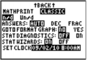
The TI-84 Plus has four graphing modes.
Func (function graphing)
Par (parametric graphing; Chapter 4)
Pol (polar graphing; Chapter 5)
Seq (sequence graphing; Chapter 6)
Other mode settings affect graphing results. Chapter 1 describes each mode setting.
Float or 0123456789 (fixed) decimal mode affects displayed graph coordinates.
Radian or Degree angle mode affects interpretation of some functions.
Connected or Dot plotting mode affects plotting of selected functions.
Sequential or Simul graphing-order mode affects function plotting when more than one function is selected.
Setting Modes from a Program
To set the graphing mode and other modes from a program, begin on a blank line in the program editor and follow these steps.
Press [MODE] to display the mode settings.
Press [down key], [right key], [left key], and [up key] to place the cursor on the mode that you want to select.
Press [ENTER] to paste the mode name to the cursor location. The mode is changed when the program is executed.
Displaying Functions in the Y= Editor
To display the Y= editor, press [Y=]. You can store up to 10 functions to the function variables Y1 through Y9, and Y0. You can graph one or more defined functions at once. In this example, functions Y1 and Y2 are defined and selected.
Defining or Editing a Function
To define or edit a function, follow these steps.
Press [Y=] to display the Y= editor.
Press [down key] to move the cursor to the function you want to define or edit. To erase a function, press [CLEAR].
Enter or edit the expression to define the function.
You may use functions and variables (including matrices and lists) in the expression.
When the expression evaluates to a nonreal number, the value is not plotted; no error is returned.
You can access the shortcut menus by pressing [ALPHA] [F1] - [F4].
The independent variable in the function is X. Func mode defines [X, T, theta, n] as X. To enter X, press [X, T, theta, n] or press [ALPHA] [X].
When you enter the first character, the = is highlighted, indicating that the function is selected.
As you enter the expression, it is stored to the variable Yn as a user-defined function in the Y= editor.
Press [ENTER] or [down key] to move the cursor to the next function.
Defining a Function from the Home Screen or a Program
To define a function from the home screen or a program, begin on a blank line and follow these steps.
Press [ALPHA] ["], enter the expression, and then press [ALPHA] ["] again.
Press [STO right arrow key].
Press [ALPHA] [F4] to display the YVAR shortcut menu, move the cursor to the function name, and then press [ENTER].
"expression" right arrow Yn
![]()
![]()
When the instruction is executed, the TI-84 Plus stores the expression to the designated variable
Yn, selects the function, and displays the message Done.
Evaluating Y= Functions in Expressions
You can calculate the value of a Y= function Yn at a specified value of X. A list of values returns a list.
Yn(value)
Yn({value1,value2,value3, . . .,value n})
Selecting and Deselecting a Function
You can select and deselect (turn on and turn off) a function in the Y= editor. A function is selected when the = sign is highlighted. The TI-84 Plus graphs only the selected functions. You can select any or all functions Y1 through Y9, and Y0.
To select or deselect a function in the Y= editor, follow these steps.
Press [Y=] to display the Y= editor.
Move the cursor to the function you want to select or deselect.
Press [left key] to place the cursor on the function’s = sign.
Press [ENTER] to change the selection status.
When you enter or edit a function, it is selected automatically. When you clear a function, it is deselected.
Turning On or Turning Off a Stat Plot in the Y= Editor
To view and change the on/off status of a stat plot in the Y= editor, use Plot1 Plot2 Plot3 (the top line of the Y= editor). When a plot is on, its name is highlighted on this line.
To change the on/off status of a stat plot from the Y= editor, press [up key] and [right key] to place the cursor on Plot1, Plot2, or Plot3, and then press [ENTER].
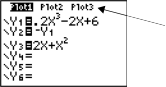
Plot1 is turned on.
Plot2 and Plot3 are turned off.
Selecting and Deselecting Functions from the Home Screen or a Program
To select or deselect a function from the home screen or a program, begin on a blank line and follow these steps.
Press [VARS] [right key] to display the VARS Y-VARS menu.
Select 4:On/Off to display the ON/OFF secondary menu.
Select 1:FnOn to turn on one or more functions or 2:FnOff to turn off one or more functions.
The instruction you select is copied to the cursor location.
Enter the number (1 through 9, or 0; not the variable Yn) of each function you want to turn on or turn off.
If you enter two or more numbers, separate them with commas.
To turn on or turn off all functions, do not enter a number after FnOn or FnOff.
FnOn[function#,function#, . . .,function n]
FnOff[function#,function#, . . .,function n]
Press [ENTER]. When the instruction is executed, the status of each function in the current mode is set and Done is displayed.
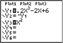
For example, in Func mode, FnOff :FnOn 1,3 turns off all functions in the Y= editor, and then turns on Y1 and Y3.
MATH Graph Style Icons in the Y= Editor
This table describes the graph styles available for function graphing. Use the styles to visually differentiate functions to be graphed together. For example, you can set Y1 as a solid line, Y2 as a dotted line, and Y3 as a thick line.
![]()
Icon Style Description
![]()
Line A solid line connects plotted points; this is the default in Connected mode
![]()
![]()
![]()
![]()
Thick A thick solid line connects plotted points Above Shading covers the area above the graph Below Shading covers the area below the graph
Path A circular cursor traces the leading edge of the graph and draws a path
![]()
Animate A circular cursor traces the leading edge of the graph without drawing a path
![]()
Dot A small dot represents each plotted point; this is the default in Dot mode
![]()
Note: Some graph styles are not available in all graphing modes. Chapters 4, 5, and 6 list the styles for Par, Pol, and Seq modes.
Setting the Graph Style
To set the graph style for a function, follow these steps.
Press [Y=] to display the Y= editor.
Press [down key] and [up key] to move the cursor to the function.
Press [left key] [left key] to move the cursor left, past the = sign, to the graph style icon in the first column. The insert cursor is displayed. (Steps 2 and 3 are interchangeable.)
Press [ENTER] repeatedly to rotate through the graph styles. The seven styles rotate in the same order in which they are listed in the table above.
Press [right key], [up key], or [down key] when you have selected a style.
Shading Above and Below
When you select above or below for two or more functions, the TI-84 Plus rotates through four shading patterns.
Vertical lines shade the first function with a above or below graph style.
Horizontal lines shade the second.
Negatively sloping diagonal lines shade the third.
Positively sloping diagonal lines shade the fourth.
The rotation returns to vertical lines for the fifth above or below function, repeating the order described above.
When shaded areas intersect, the patterns overlap.
Note: When above or below is selected for a Y= function that graphs a family of curves, such as
Y1={1,2,3}X, the four shading patterns rotate for each member of the family of curves.
Setting a Graph Style from a Program
To set the graph style from a program, select H:GraphStyle( from the PRGM CTL menu. To display this menu, press [PRGM] while in the program editor. function# is the number of the Y= function name in the current graphing mode. graphstyle# is an integer from 1 to 7 that corresponds to the graph style, as shown below.
1 = line
2 = thick
3 = above
4 = below
5 = path
6 = animate
7 = dot
GraphStyle(function#,graphstyle#)
For example, when this program is executed in Func mode, GraphStyle(1,3) sets Y1 to above.
The TI-84 Plus Viewing Window
The viewing window is the portion of the coordinate plane defined by Xmin, Xmax, Ymin, and Ymax. Xscl (X scale) defines the distance between tick marks on the x-axis. Yscl (Y scale) defines the distance between tick marks on the y-axis. To turn off tick marks, set Xscl=0 and Yscl=0.
Displaying the Window Variables
To display the current window variable values, press [WINDOW]. The window editor above and to the right shows the default values in Func graphing mode and Radian angle mode. The window variables differ from one graphing mode to another.
Xres sets pixel resolution (1 through 8) for function graphs only. The default is 1.
At Xres=1, functions are evaluated and graphed at each pixel on the x-axis.
At Xres=8, functions are evaluated and graphed at every eighth pixel along the x-axis.
Note: Small Xres values improve graph resolution but may cause the TI-84 Plus to draw graphs more slowly.
Changing a Window Variable Value
To change a window variable value from the window editor, follow these steps.
Press [down key] or [up key] to move the cursor to the window variable you want to change.
Edit the value, which can be an expression.
Enter a new value, which clears the original value.
Move the cursor to a specific digit, and then edit it.
Press [ENTER], [down key], or [up key]. If you entered an expression, the TI-84 Plus evaluates it. The new value is stored.
Note: Xmin<Xmax and Ymin<Ymax must be true in order to graph.
Storing to a Window Variable from the Home Screen or a Program
To store a value, which can be an expression, to a window variable, begin on a blank line and follow these steps.
Enter the value you want to store.
Press [STO right arrow].
Press [VARS] to display the VARS menu.
Select 1:Window to display the Func window variables (X/Y secondary menu).
Press [right key] to display the Par and Pol window variables (T/ theta secondary menu).
Press [right key] [right key] to display the Seq window variables (U/V/W secondary menu).
Select the window variable to which you want to store a value. The name of the variable is pasted to the current cursor location.
Press [ENTER] to complete the instruction.
When the instruction is executed, the TI-84 Plus stores the value to the window variable and displays the value.
![]()
DeltaX and DeltaY
The variables DeltaX and DeltaY (items 8 and 9 on the VARS (1:Window) X/Y secondary menu; DeltaX is also on the Window screen) define the distance from the center of one pixel to the center of any adjacent pixel on a graph (graphing accuracy). DeltaX and DeltaY are calculated from Xmin, Xmax, Ymin, and Ymax when you display a graph.
ï„X =
Xmax – Xmin
--------------------------------------
94
ï„Y =
Ymax – Ymin
--------------------------------------
62
You can store values to DeltaX and DeltaY. If you do, Xmax and Ymax are calculated from DeltaX,
Xmin, DeltaY, and Ymin.
Note: The ZFrac ZOOM settings (Zfrac1/2, ZFrac1/3, ZFrac1/4, ZFrac1/5, ZFrac1/8, ZFrac1/10) change DeltaX and DeltaY to fractional values. If fractions are not needed for your problem, you can adjust DeltaX and DeltaY to suit your needs.
Displaying the Format Settings
To display the format settings, press [2nd] [FORMAT]. The default settings are highlighted below.
Note: You can also go to the Format Graph screen from the Mode screen by selecting YES at the GoTo Format Graph prompt. After you make changes, press [MODE] to return to the Mode screen.
![]()
RectGC PolarGC Sets cursor coordinates. CoordOn CoordOff Sets coordinates display on or off. GridOff GridOn Sets grid off or on.
AxesOn AxesOff Sets axes on or off.
![]()
![]()
LabelOff LabelOn Sets axes label off or on.
ExprOn ExprOff Sets expression display on or off.
![]()
Format settings define a graph’s appearance on the display. Format settings apply to all graphing modes. Seq graphing mode has an additional mode setting (Chapter 6).
Changing a Format Setting
To change a format setting, follow these steps.
Press [down key], [right key], [up key], and [left key] as necessary to move the cursor to the setting you want to select.
Press [ENTER] to select the highlighted setting.
RectGC, PolarGC
RectGC (rectangular graphing coordinates) displays the cursor location as rectangular coordinates X and Y.
PolarGC (polar graphing coordinates) displays the cursor location as polar coordinates R and theta. The RectGC/PolarGC setting determines which variables are updated when you plot the graph,
move the free-moving cursor, or trace.
RectGC updates X and Y; if CoordOn format is selected, X and Y are displayed.
PolarGC updates X, Y, R, and theta; if CoordOn format is selected, R and theta are displayed.
CoordOn, CoordOff
CoordOn (coordinates on) displays the cursor coordinates at the bottom of the graph. If ExprOff
format is selected, the function number is displayed in the top-right corner.
CoordOff (coordinates off) does not display the function number or coordinates.
GridOff, GridOn
Grid points cover the viewing window in rows that correspond to the tick marks on each axis.
GridOff does not display grid points.
GridOn displays grid points.
AxesOn, AxesOff
AxesOn displays the axes.
AxesOff does not display the axes.
This overrides the LabelOff/LabelOn format setting.
LabelOff, LabelOn
LabelOff and LabelOn determine whether to display labels for the axes (X and Y), if AxesOn format is also selected.
ExprOn, ExprOff
ExprOn and ExprOff determine whether to display the Y= expression when the trace cursor is active. This format setting also applies to stat plots.
When ExprOn is selected, the expression is displayed in the top-left corner of the graph screen. When ExprOff and CoordOn both are selected, the number in the top-right corner specifies which
function is being traced.
Displaying a New Graph
To display the graph of the selected function or functions, press [GRAPH]. TRACE, ZOOM instructions, and CALC operations display the graph automatically. As the TI-84 Plus plots the graph, the busy indicator is on. As the graph is plotted, X and Y are updated.
Pausing or Stopping a Graph
While plotting a graph, you can pause or stop graphing.
Press [ENTER] to pause; then press [ENTER] to resume.
Press [ON] to stop; then press [GRAPH] to redraw.
Smart Graph
Smart Graph is a TI-84 Plus feature that redisplays the last graph immediately when you press [GRAPH], but only if all graphing factors that would cause replotting have remained the same since the graph was last displayed.
If you performed any of the following actions since the graph was last displayed, the TI-84 Plus will replot the graph based on new values when you press [GRAPH].
Changed a mode setting that affects graphs
Changed a function in the current picture
Selected or deselected a function or stat plot
Changed the value of a variable in a selected function
Changed a window variable or graph format setting
Cleared drawings by selecting ClrDraw
Changed a stat plot definition
Overlaying Functions on a Graph
On the TI-84 Plus, you can graph one or more new functions without replotting existing functions. For example, store sin(X) to Y1 in the Y= editor and press [GRAPH]. Then store cos(X) to Y2 and press [GRAPH] again. The function Y2 is graphed on top of Y1, the original function.
Graphing a Family of Curves
If you enter a list (Chapter 11) as an element in an expression, the TI-84 Plus plots the function for each value in the list, thereby graphing a family of curves. In Simul graphing-order mode, it graphs all functions sequentially for the first element in each list, and then for the second, and so on.
{2,4,6}sin(X) graphs three functions: 2 sin(X), 4 sin(X), and 6 sin(X).
{2,4,6}sin({1,2,3}X) graphs 2 sin(X), 4 sin(2X), and 6 sin(3X).
Note: When using more than one list, the lists must have the same dimensions.
Free-Moving Cursor
When a graph is displayed, press [left key], [right key], [up key], or [down key] to move the cursor around the graph. When you first display the graph, no cursor is visible. When you press [left key], [right key], [up key], or [down key], the cursor moves from the center of the viewing window.
As you move the cursor around the graph, the coordinate values of the cursor location are displayed at the bottom of the screen if CoordOn format is selected. The Float/Fix decimal mode setting determines the number of decimal digits displayed for the coordinate values.
To display the graph with no cursor and no coordinate values, press [CLEAR] or [ENTER]. When you press [left key], [right key], [up key], or [down key], the cursor moves from the same position.
Graphing Accuracy
The free-moving cursor moves from pixel to pixel on the screen. When you move the cursor to a pixel that appears to be on the function, the cursor may be near, but not actually on, the function. The coordinate value displayed at the bottom of the screen actually may not be a point on the function. To move the cursor along a function, use [TRACE].
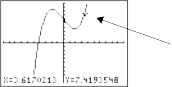
The coordinate values displayed as you move the cursor approximate actual math coordinates, accurate to within the width and height of the pixel. As Xmin, Xmax, Ymin, and Ymax get closer together (as in a Zoom In) graphing accuracy increases, and the coordinate values more closely approximate the math coordinates.
Free- moving cursor appears to be on the curve
Beginning a Trace
Use TRACE to move the cursor from one plotted point to the next along a function. To begin a trace, press [TRACE]. If the graph is not displayed already, press [TRACE] to display it. The trace cursor is on the first selected function in the Y= editor, at the middle X value on the screen. The cursor coordinates are displayed at the bottom of the screen if CoordOn format is selected. The Y= expression is displayed in the top-left corner of the screen, if ExprOn format is selected.
Moving the Trace Cursor
![]()
To move the TRACE cursor do this:
![]()
![]()
To the previous or next plotted point, press [left key] or [right key].
Five plotted points on a function (Xres affects this),
press [2nd] [left key] or [2nd] [right key].
![]()
![]()
![]()
To any valid X value on a function, enter a value, and then press [ENTER]. From one function to another, press [up key] or [down key].
When the trace cursor moves along a function, the Y value is calculated from the X value; that is,
Y=Yn(X). If the function is undefined at an X value, the Y value is blank.
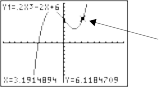 Trace cursor on the curve
If you move the trace cursor beyond the top or bottom of the screen, the coordinate values at the bottom of the screen continue to change appropriately.
Moving the Trace Cursor from Function to Function
To move the trace cursor from function to function, press [down key] and [up key]. The cursor follows the order of the selected functions in the Y= editor. The trace cursor moves to each function at the same X value. If ExprOn format is selected, the expression is updated.
Moving the Trace Cursor to Any Valid X Value
To move the trace cursor to any valid X value on the current function, enter the value. When you enter the first digit, an X= prompt and the number you entered are displayed in the bottom-left corner of the screen. You can enter an expression at the X= prompt. The value must be valid for the current viewing window. When you have completed the entry, press [ENTER] to move the cursor.
Note: This feature does not apply to stat plots.
Panning to the Left or Right
If you trace a function beyond the left or right side of the screen, the viewing window automatically pans to the left or right. Xmin and Xmax are updated to correspond to the new viewing window.
Quick Zoom
While tracing, you can press [ENTER] to adjust the viewing window so that the cursor location becomes the center of the new viewing window, even if the cursor is above or below the display. This allows panning up and down. After Quick Zoom, the cursor remains in TRACE.
Leaving and Returning to TRACE
When you leave and return to TRACE, the trace cursor is displayed in the same location it was in when you left TRACE, unless Smart Graph has replotted the graph.
Using TRACE in a Program
On a blank line in the program editor, press [TRACE]. The instruction Trace is pasted to the cursor location. When the instruction is encountered during program execution, the graph is displayed with the trace cursor on the first selected function. As you trace, the cursor coordinate values are updated. When you finish tracing the functions, press [ENTER] to resume program execution.
ZOOM Menu
To display the ZOOM menu, press [ZOOM]. You can adjust the viewing window of the graph quickly in several ways. All ZOOM instructions are accessible from programs.
![]()
![]()
ZOOM MEMORY
|
1: |
ZBox |
Draws a box to define the viewing window. |
|
2: |
Zoom In |
Magnifies the graph around the cursor. |
|
3: |
Zoom Out |
Views more of a graph around the cursor. |
|
4: |
ZDecimal |
Sets DeltaX and DeltaY to 0.1. |
|
5: |
ZSquare |
Sets equal-size pixels on the X and Y axes. |
|
6: |
ZStandard |
Sets the standard window variables. |
|
7: |
ZTrig |
Sets the built-in trig window variables. |
|
8: |
ZInteger |
Sets integer values on the X and Y axes. |
|
9: |
ZoomStat |
Sets the values for current stat lists. |
|
0: |
ZoomFit |
Fits YMin and YMax between XMin and XMax. |
|
A: |
ZQuadrant1 |
Displays the portion of the graph that is in quadrant 1 |
![]()
ZOOM MEMORY
|
B: |
ZFrac1/2 |
Sets the window variables so that you can trace in increments of 1/2, if possible. Sets DeltaX and DeltaY to 1/2. |
|
C: |
ZFrac1/3 |
Sets the window variables so that you can trace in increments of 1/3, if possible. Sets DeltaX and DeltaY to 1/3. |
|
D: |
ZFrac1/4 |
Sets the window variables so that you can trace in increments of 1/4, if possible. Sets DeltaX and DeltaY to 1/4. |
|
E: |
ZFrac1/5 |
Sets the window variables so that you can trace in increments of 1/5, if possible. Sets DeltaX and DeltaY to 1/5. |
|
F: |
ZFrac1/8 |
Sets the window variables so that you can trace in increments of 1/8, if possible. Sets DeltaX and DeltaY to 1/8. |
|
G: |
ZFrac1/10 |
Sets the window variables so that you can trace in increments of 1/10, if possible. Sets DeltaX and DeltaY to 1/10. |
Note: You can adjust all window variables from the VARS menu by pressing [VARS] 1:Window and then selecting the variable from the X/Y, T/theta, or U/V/W menu.
Zoom Cursor
When you select 1:ZBox, 2:Zoom In, or 3:Zoom Out, the cursor on the graph becomes the zoom cursor (+), a smaller version of the free-moving cursor (+).
ZBox
To define a new viewing window using ZBox, follow these steps.
Select 1:ZBox from the ZOOM menu. The zoom cursor is displayed at the center of the screen.
Move the zoom cursor to any spot you want to define as a corner of the box, and then press [ENTER]. When you move the cursor away from the first defined corner, a small, square dot indicates the spot.
Press [left key], [up key], [right key], or [down key]. As you move the cursor, the sides of the box lengthen or shorten proportionately on the screen.
Note: To cancel ZBox before you press [ENTER], press [CLEAR].
When you have defined the box, press [ENTER] to replot the graph.
To use ZBox to define another box within the new graph, repeat steps 2 through 4. To cancel ZBox, press [CLEAR].
Zoom In, Zoom Out
Zoom In magnifies the part of the graph that surrounds the cursor location. Zoom Out displays a greater portion of the graph, centered on the cursor location. The XFact and YFact settings determine the extent of the zoom.
To zoom in on a graph, follow these steps.
Check XFact and YFact; change as needed.
Select 2:Zoom In from the ZOOM menu. The zoom cursor is displayed.
Move the zoom cursor to the point that is to be the center of the new viewing window.
Press [ENTER]. The TI-83 Plus adjusts the viewing window by XFact and YFact; updates the window variables; and replots the selected functions, centered on the cursor location.
Zoom in on the graph again in either of two ways.
To zoom in at the same point, press [ENTER].
To zoom in at a new point, move the cursor to the point that you want as the center of the new viewing window, and then press [ENTER].
To zoom out on a graph, select 3:Zoom Out and repeat steps 3 through 5. To cancel Zoom In or Zoom Out, press [CLEAR].
ZDecimal
ZDecimal replots the functions immediately. It updates the window variables to preset values, as shown below. These values set DeltaX and DeltaY equal to 0.1 and set the X and Y value of each pixel to one decimal place.
Xmin=-4.7 Xmax=4.7 Xscl=1
Ymin=-3.1 Ymax=3.1 Yscl=1
ZSquare
ZSquare replots the functions immediately. It redefines the viewing window based on the current values of the window variables. It adjusts in only one direction so that DeltaX=DeltaY, which makes the graph of a circle look like a circle. Xscl and Yscl remain unchanged. The midpoint of the current graph (not the intersection of the axes) becomes the midpoint of the new graph.
ZStandard
ZStandard replots the functions immediately. It updates the window variables to the standard values shown below.
Xmin=-10 Xmax=10 Xscl=1
Ymin=-10 Ymax=10 Yscl=1
Xres=1
ZTrig
ZTrig replots the functions immediately. It updates the window variables to preset values that are appropriate for plotting trig functions. Those preset values in Radian mode are shown below.
Xmin=-(47/24)pi (decimal equivalent) Xmax=(47/24)pi (decimal equivalent) Xscl=pi/2 (decimal equivalent)
Ymin=-4 Ymax=4 Yscl=1
ZInteger
ZInteger redefines the viewing window to the dimensions shown below. To use ZInteger, move the cursor to the point that you want to be the center of the new window, and then press [ENTER]; ZInteger replots the functions.
DeltaX=1 DeltaY=1
Xscl=10 Yscl=10
ZoomStat
ZoomStat redefines the viewing window so that all statistical data points are displayed. For regular and modified box plots, only Xmin and Xmax are adjusted.
ZoomFit
ZoomFit replots the functions immediately. ZoomFit recalculates YMin and YMax to include the minimum and maximum Y values of the selected functions between the current XMin and XMax. XMin and XMax are not changed.
ZQuadrant1
ZQuandrant1 replots the function immediately. It redefines the window settings so that only quadrant 1 is displayed.
ZFrac1/2
ZFrac1/2 replots the functions immediately. It updates the window variables to preset values, as shown below. These values set DeltaX and DeltaY equal to 1/2 and set the X and Y value of each pixel to one decimal place.
Xmin=-47/2 Xmax=47/2 Xscl=1
Ymin=-31/2 Ymax=31/2 Yscl=1
ZFrac1/3
ZFrac1/3 replots the functions immediately. It updates the window variables to preset values, as shown below. These values set DeltaX and DeltaY equal to 1/3 and set the X and Y value of each pixel to one decimal place.
Xmin=-47/3 Xmax=47/3 Xscl=1
Ymin=-31/3 Ymax=31/3 Yscl=1
ZFrac1/4
ZFrac1/4 replots the functions immediately. It updates the window variables to preset values, as shown below. These values set DeltaX and DeltaY equal to 1/4 and set the X and Y value of each pixel to one decimal place.
Xmin=-47/4 Xmax=47/4 Xscl=1
Ymin=-31/4 Ymax=31/4 Yscl=1
ZFrac1/5
ZFrac1/5 replots the functions immediately. It updates the window variables to preset values, as shown below. These values set DeltaX and DeltaY equal to 1/5 and set the X and Y value of each pixel to one decimal place.
Xmin=-47/5 Xmax=47/5 Xscl=1
Ymin=-31/5 Ymax=31/5 Yscl=1
ZFrac1/8
ZDecimal replots the functions immediately. It updates the window variables to preset values, as shown below. These values set DeltaX and DeltaY equal to 1/8 and set the X and Y value of each pixel to one decimal place.
Xmin=-47/8 Xmax=47/8 Xscl=1
Ymin=-31/8 Ymax=31/8 Yscl=1
ZFrac1/10
ZFrac1/10 replots the functions immediately. It updates the window variables to preset values, as shown below. These values set DeltaX and DeltaY equal to 1/10 and set the X and Y value of each pixel to one decimal place.
Xmin=-47/10 Xmax=47/10 Xscl=1
Ymin=-31/10 Ymax=31/10 Yscl=1
ZOOM MEMORY Menu
To display the ZOOM MEMORY menu, press [ZOOM] [right key].
![]()
ZOOM MEMORY
|
1: |
ZPrevious |
Uses the previous viewing window. |
|
2: |
ZoomSto |
Stores the user-defined window. |
|
3: |
ZoomRcl |
Recalls the user-defined window. |
|
4: |
SetFactors... |
Changes Zoom In and Zoom Out factors. |
![]()
ZPrevious
ZPrevious replots the graph using the window variables of the graph that was displayed before you executed the last ZOOM instruction.
ZoomSto
ZoomSto immediately stores the current viewing window. The graph is displayed, and the values of the current window variables are stored in the user-defined ZOOM variables ZXmin, ZXmax, ZXscl, ZYmin, ZYmax, ZYscl, and ZXres.
These variables apply to all graphing modes. For example, changing the value of ZXmin in Func mode also changes it in Par mode.
ZoomRcl
ZoomRcl graphs the selected functions in a user-defined viewing window. The user-defined viewing window is determined by the values stored with the ZoomSto instruction. The window variables are updated with the user-defined values, and the graph is plotted.
ZOOM FACTORS
The zoom factors, XFact and YFact, are positive numbers (not necessarily integers) greater than or equal to 1. They define the magnification or reduction factor used to Zoom In or Zoom Out around a point.
Checking XFact and YFact
To display the ZOOM FACTORS screen, where you can review the current values for XFact and
YFact, select 4:SetFactors from the ZOOM MEMORY menu. The values shown are the defaults.
![]()
Changing XFact and YFact
You can change XFact and YFact in either of two ways.
Enter a new value. The original value is cleared automatically when you enter the first digit.
Place the cursor on the digit you want to change, and then enter a value or press [DEL] to delete it.
Using ZOOM MEMORY Menu Items from the Home Screen or a Program
From the home screen or a program, you can store directly to any of the user-defined ZOOM variables.
![]()
From a program, you can select the ZoomSto and ZoomRcl instructions from the ZOOM MEMORY
menu.
CALCULATE Menu
To display the CALCULATE menu, press [2nd] [CALC]. Use the items on this menu to analyze the current graph functions.
![]()
CALCULATE
1: value Calculates a function Y value for a given X. 2: zero Finds a zero (x-intercept) of a function. 3: minimum Finds a minimum of a function.
4: maximum Finds a maximum of a function.
5: intersect Finds an intersection of two functions.
6: dy/dx Finds a numeric derivative of a function.
7: Numerical
integral
Finds a numeric integral of a function.
![]()
value
value evaluates one or more currently selected functions for a specified value of X.
Note: When a value is displayed for X, press [CLEAR] to clear the value. When no value is displayed, press [CLEAR] to cancel the value operation.
To evaluate a selected function at X, follow these steps.
Select 1:value from the CALCULATE menu. The graph is displayed with X= in the bottom-left corner.
Enter a real value, which can be an expression, for X between Xmin and Xmax.
Press [ENTER].
The cursor is on the first selected function in the Y= editor at the X value you entered, and the coordinates are displayed, even if CoordOff format is selected.
To move the cursor from function to function at the entered X value, press [up key] or [down key]. To restore the free-moving cursor, press [left key] or [right key].
zero
zero finds a zero (x-intercept or root) of a function using solve(. Functions can have more than one x-intercept value; zero finds the zero closest to your guess.
The time zero spends to find the correct zero value depends on the accuracy of the values you specify for the left and right bounds and the accuracy of your guess.
To find a zero of a function, follow these steps.
Select 2:zero from the CALCULATE menu. The current graph is displayed with Left Bound? in the bottom-left corner.
Press [up key]or [down key] to move the cursor onto the function for which you want to find a zero.
Press [left key] or [right key] (or enter a value) to select the x-value for the left bound of the interval, and then press [ENTER]. A â–º (right triangle) indicator on the graph screen shows the left bound. Right Bound? is displayed in the bottom-left corner. Press [left key] or [right key](or enter a value) to select the x-value for the right bound, and then press [ENTER]. A â—„ (left triangle) indicator on the graph screen shows the right bound. Guess? is then displayed in the bottom-left corner.
Press [left key] or [right key] (or enter a value) to select a point near the zero of the function, between the bounds, and then press [ENTER].
The cursor is on the solution and the coordinates are displayed, even if CoordOff format is selected. To move to the same x-value for other selected functions, press [up key] or [down key]. To restore the free-moving cursor, press [left key] or [right key].
minimum, maximum
minimum and maximum find a minimum or maximum of a function within a specified interval to a tolerance of 1E-5.
To find a minimum or maximum, follow these steps.
Select 3:minimum or 4:maximum from the CALCULATE menu. The current graph is displayed.
Select the function and set left bound, right bound, and guess as described for zero.
The cursor is on the solution, and the coordinates are displayed, even if you have selected
CoordOff format; Minimum or Maximum is displayed in the bottom-left corner.
To move to the same x-value for other selected functions, press [up key] or [down key]. To restore the free-moving cursor, press [left key] or [right key].
intersect
intersect finds the coordinates of a point at which two or more functions intersect using solve(. The intersection must appear on the display to use intersect.
To find an intersection, follow these steps.
Select 5:intersect from the CALCULATE menu. The current graph is displayed with
First curve? in the bottom-left corner.
Press [down key] or [up key], if necessary, to move the cursor to the first function, and then press [ENTER]. Second curve? is displayed in the bottom-left corner.
Press [down key] or [up key], if necessary, to move the cursor to the second function, and then press [ENTER].
Press [right key] or [left key] to move the cursor to the point that is your guess as to location of the intersection, and then press [ENTER].
The cursor is on the solution and the coordinates are displayed, even if CoordOff format is selected. Intersection is displayed in the bottom-left corner. To restore the free-moving cursor, press [left key], [up key], [right key], or [down key].
dy/dx
dy/dx (numerical derivative) finds the numerical derivative (slope) of a function at a point, with
epsilon=1E-3.
To find a function’s slope at a point, follow these steps.
Select 6:dy/dx from the CALCULATE menu. The current graph is displayed.
Press [up key] or [down key] to select the function for which you want to find the numerical derivative.
Press [left key] or [right key] (or enter a value) to select the X value at which to calculate the derivative, and then press [ENTER].
The cursor is on the solution and the numerical derivative is displayed.
To move to the same x-value for other selected functions, press [up key] or [down key]. To restore the free-moving cursor, press [left key] or [right key].
Numerical Integral
Numerical integral finds the numerical integral of a function in a specified interval. It uses the fnInt(
function, with a tolerance of epsilon=1E-3.
To find the numerical integral of a function, follow these steps.
Select 7:numerical integral from the CALCULATE menu. The current graph is displayed with
Lower Limit? in the bottom-left corner.
Press [up key] or [down key] to move the cursor to the function for which you want to calculate the integral.
Set lower and upper limits as you would set left and right bounds for zero. The integral value is displayed, and the integrated area is shaded.
Note: The shaded area is a drawing. Use ClrDraw (Chapter 8) or any action that invokes Smart Graph to clear the shaded area.
Getting Started is a fast-paced introduction. Read the chapter for details.
Graph the parametric equation that describes the path of a ball hit at an initial speed of 30 meters per second, at an initial angle of 25 degrees with the horizontal from ground level. How far does the ball travel? When does it hit the ground? How high does it go? Ignore all forces except gravity.
For initial velocity vo and angle theta, the position of the ball as a function of time has horizontal and vertical components.
Horizontal: X1(t)=tv0cos(theta) Vertical: Y1(t)=tv0sin(theta)- 1/2 gtsquared
The vertical and horizontal vectors of the ball’s motion also will be graphed.
Vertical vector: Horizontal vector:
Gravity constant:
X2(t)=0 X3(t)=X1(t)
g=9.8 m/sec squared
Y2(t)=Y1(t) Y3(t)=0
Press [MODE]. Press [down key] [down key] [down key] [right key] [ENTER] to select Par mode. Press [down key] [down key] [right key] [ENTER] to select Simul for simultaneous graphing of all three parametric equations in this example.
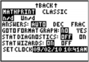
Press [down key] [down key] [down key] [down key] [down key] [down key] [right key] [ENTER] to go to the Format Graph screen. Press [down key] [down key] [down key] [right key] [ENTER] to select AxesOff, which turns off the axes.
Press [Y=]. Press 30 [X, T, theta, n] [COS] 25 [2nd] [ANGLE] 1 (to select °) [ ) ] [ENTER] to define X1T in terms of T.
Press [X, T, theta, n] [SIN] 25 [2nd] [ANGLE] 1 [)]
[-] [ALPHA] [F1] 1 (to select n/d) 9.8 [right key] 2 [right key] [X, T, theta, n] [x squared][ENTER] to define Y1T.
The vertical component vector is defined by X2T
and Y2T.
Press 0 [ENTER] to define X2T.
Press [ALPHA][F4][down key] [ENTER] [ENTER]
to define Y2T.
The horizontal component vector is defined by X3T
and Y3T.
Press [ALPHA][F4][ENTER] [ENTER] to define
X3T.
Press 0 [ENTER] to define Y3T.
Press [left key] [left key] [up key] [ENTER] to change the graph style to Thick for X3T and Y3T. Press [up key] [ENTER] [ENTER] to change the graph style to Path for X2T and Y2T. Press [up key] [ENTER] [ENTER] to change the graph style to Path for X1T and Y1T. (These keystrokes assume that all graph styles were set to Line originally.)
Press [WINDOW]. Enter these values for the window variables.
|
Tmin=0 |
Xmin=-10 |
Ymin=-5 |
|
Tmax=5 |
Xmax=100 |
Ymax=15 |
|
Tstep=.1 |
Xscl=50 |
Yscl=10 |
Note: You can check all WINDOW variables, including DeltaX and DeltaY by pressing [VARS] 1:Window.
Press [GRAPH]. The plotting action simultaneously shows the ball in flight and the vertical and horizontal component vectors of the motion.
Note: To simulate the ball flying through the air, set graph style to Animate for X1T and Y1T.
Press [TRACE] to obtain numerical results and answer the questions at the beginning of this section.
Tracing begins at Tmin on the first parametric equation (X1T and Y1T). As you press [right key] to trace the curve, the cursor follows the path of the ball over time. The values for X (distance), Y (height), and T (time) are displayed at the bottom of the screen.
TI-84 Plus Graphing Mode Similarities
The steps for defining a parametric graph are similar to the steps for defining a function graph. Chapter 4 assumes that you are familiar with Chapter 3: Function Graphing. Chapter 4 details aspects of parametric graphing that differ from function graphing.
Setting Parametric Graphing Mode
To display the mode screen, press [MODE]. To graph parametric equations, you must select parametric graphing mode before you enter window variables and before you enter the components of parametric equations.
Displaying the Parametric Y= Editor
After selecting parametric graphing mode, press [Y=] to display the parametric Y= editor.
In this editor, you can display and enter both the X and Y components of up to six equations, X1T and Y1T through X6T and Y6T. Each is defined in terms of the independent variable T. A common application of parametric graphs is graphing equations over time.
Selecting a Graph Style
The icons to the left of X1T through X6T represent the graph style of each parametric equation. The default in parametric mode is line, which connects plotted points. Line, thick, path, animate, and dot styles are available for parametric graphing.
Defining and Editing Parametric Equations
To define or edit a parametric equation, follow the steps in Chapter 3 for defining a function or editing a function. The independent variable in a parametric equation is T. In parametric graphing mode, you can enter the parametric variable T in either of two ways.
Press [X,T, theta, n].
Press [ALPHA] [T].
Two components, X and Y, define a single parametric equation. You must define both of them.
Selecting and Deselecting Parametric Equations
The TI-84 Plus graphs only the selected parametric equations. In the Y= editor, a parametric equation is selected when the = signs of both the X and Y components are highlighted. You may select any or all of the equations X1T and Y1T through X6T and Y6T.
To change the selection status, move the cursor onto the = sign of either the X or Y component and press [ENTER]. The status of both the X and Y components is changed.
Setting Window Variables
To display the window variable values, press [WINDOW]. These variables define the viewing window. The values below are defaults for parametric graphing in Radian angle mode.
![]()
Tmin=0 Smallest T value to evaluate Tmax=6.2831853... Largest T value to evaluate (2pi) Tstep=.1308996... T value increment (pi24) Xmin=-10 Smallest X value to be displayed
Xmax=10 Largest X value to be displayed
Xscl=1 Spacing between the X tick marks
Ymin=-10 Smallest Y value to be displayed
Ymax=10 Largest Y value to be displayed
Yscl=1 Spacing between the Y tick marks
![]()
Note: To ensure that sufficient points are plotted, you may want to change the T window variables.
Setting the Graph Format
To display the current graph format settings, press [2nd] [FORMAT]. Chapter 3 describes the format settings in detail. The other graphing modes share these format settings; Seq graphing mode has an additional axes format setting.
Displaying a Graph
When you press [GRAPH], the TI-84 Plus plots the selected parametric equations. It evaluates the X and Y components for each value of T (from Tmin to Tmax in intervals of Tstep), and then plots each point defined by X and Y. The window variables define the viewing window.
As the graph is plotted, X, Y, and T are updated. Smart Graph applies to parametric graphs.
Window Variables and Y-VARS Menus
You can perform these actions from the home screen or a program.
Access functions by using the name of the X or Y component of the equation as a variable.
![]()
Store parametric equations.
Select or deselect parametric equations.
Store values directly to window variables.
![]()
Free-Moving Cursor
The free-moving cursor in parametric graphing works the same as in Func graphing.
In RectGC format, moving the cursor updates the values of X and Y; if CoordOn format is selected, X and Y are displayed.
In PolarGC format, X, Y, R, and theta are updated; if CoordOn format is selected, R and theta are displayed.
TRACE
To activate TRACE, press [TRACE]. When TRACE is active, you can move the trace cursor along the graph of the equation one Tstep at a time. When you begin a trace, the trace cursor is on the first selected function at Tmin. If ExprOn is selected, then the function is displayed.
In RectGC format, TRACE updates and displays the values of X, Y, and T if CoordOn format is on. In PolarGC format, X, Y, R, theta and T are updated; if CoordOn format is selected, R, theta, and T
are displayed. The X and Y (or R and theta) values are calculated from T.
To move five plotted points at a time on a function, press [2nd] [left key] or [2nd] [right key]. If you move the cursor beyond the top or bottom of the screen, the coordinate values at the bottom of the screen continue to change appropriately.
Quick Zoom is available in parametric graphing; panning is not.
Moving the Trace Cursor to Any Valid T Value
To move the trace cursor to any valid T value on the current function, enter the number. When you enter the first digit, a T= prompt and the number you entered are displayed in the bottom-left corner of the screen. You can enter an expression at the T= prompt. The value must be valid for the current viewing window. When you have completed the entry, press [ENTER] to move the cursor.
![]()
ZOOM
ZOOM operations in parametric graphing work the same as in Func graphing. Only the X (Xmin,
Xmax, and Xscl) and Y (Ymin, Ymax, and Yscl) window variables are affected.
The T window variables (Tmin, Tmax, and Tstep) are only affected when you select ZStandard. The VARS ZOOM secondary menu ZT/Ztheta items 1:ZTmin, 2:ZTmax, and 3:ZTstep are the zoom memory variables for parametric graphing.
CALC
CALC operations in parametric graphing work the same as in Func graphing. The CALCULATE
menu items available in parametric graphing are 1:value, 2:dy/dx, 3:dy/dt, and 4:dx/dt.
Getting Started is a fast-paced introduction. Read the chapter for details.
The polar equation R=Asin(Btheta) graphs a rose. Graph the rose for A=8 and B=2.5, and then explore the appearance of the rose for other values of A and B.
Press [MODE] to display the MODE screen. Press [down key] [down key] [down key] [right key][right key] [right key] [ENTER] to select Pol graphing mode. Select the defaults (the options on the left) for the other mode settings.
Press [Y=] to display the polar Y= editor. Press 8
[SIN] 2.5 [X,T, theta, n] [)] [ENTER] to define r1.
Press [ZOOM] 6 to select 6:ZStandard and graph the equation in the standard viewing window. The graph shows only five petals of the rose, and the rose does not appear to be symmetrical. This is because the standard window sets thetamax=2pi and defines the window, rather than the pixels, as square.
Press [WINDOW] to display the window variables.
Press [down key] 4 [2nd] [pi] to increase the value of thetamax to 4pi.
Press [ZOOM] 5 to select 5:ZSquare and plot the graph.
Repeat steps 2 through 5 with new values for the variables A and B in the polar equation r1=Asin(Btheta). Observe how the new values affect the graph.
TI-84 Plus Graphing Mode Similarities
The steps for defining a polar graph are similar to the steps for defining a function graph. Chapter 5 assumes that you are familiar with Chapter 3: Function Graphing. Chapter 5 details aspects of polar graphing that differ from function graphing.
Setting Polar Graphing Mode
To display the mode screen, press [MODE]. To graph polar equations, you must select Pol graphing mode before you enter values for the window variables and before you enter polar equations.
Displaying the Polar Y= Editor
After selecting Pol graphing mode, press [Y=] to display the polar Y= editor.
In this editor, you can enter and display up to six polar equations, r1 through r6. Each is defined in terms of the independent variable theta.
Selecting Graph Styles
The icons to the left of r1 through r6 represent the graph style of each polar equation. The default in Pol graphing mode is line, which connects plotted points. Line, thick, path, animate, and dot styles are available for polar graphing.
Defining and Editing Polar Equations
To define or edit a polar equation, follow the steps in Chapter 3 for defining a function or editing a function. The independent variable in a polar equation is theta. In Pol graphing mode, you can enter the polar variable theta in either of two ways.
Press [X,T, theta, n].
Press [ALPHA] [theta].
Selecting and Deselecting Polar Equations
The TI-84 Plus graphs only the selected polar equations. In the Y= editor, a polar equation is selected when the = sign is highlighted. You may select any or all of the equations.
To change the selection status, move the cursor onto the = sign, and then press [ENTER].
Setting Window Variables
To display the window variable values, press [WINDOW]. These variables define the viewing window. The values below are defaults for Pol graphing in Radian angle mode.
![]()
thetamin=0 Smallest theta value to evaluate thetamax=6.2831853... Largest theta value to evaluate (2pi) thetastep=.1308996... Increment between theta values (pi/24) Xmin=-10 Smallest X value to be displayed
Xmax=10 Largest X value to be displayed
Xscl=1 Spacing between the X tick marks
Ymin=-10 Smallest Y value to be displayed
Ymax=10 Largest Y value to be displayed
Yscl=1 Spacing between the Y tick marks
![]()
Note: To ensure that sufficient points are plotted, you may want to change the theta window variables.
Setting the Graph Format
To display the current graph format settings, press [2nd] [FORMAT]. Chapter 3 describes the format settings in detail. The other graphing modes share these format settings.
Displaying a Graph
When you press [GRAPH], the TI-84 Plus plots the selected polar equations. It evaluates R for each value of theta (from thetamin to thetamax in intervals of thetastep) and then plots each point. The window variables define the viewing window.
As the graph is plotted, X, Y, R, and theta are updated. Smart Graph applies to polar graphs.
Window Variables and Y-VARS Menus
You can perform these actions from the home screen or a program.
Access functions by using the name of the equation as a variable. These function names are available on the YVARS shortcut menu ([ALPHA][F4]).
![]()
Store polar equations.
![]()
![]()
Select or deselect polar equations.
![]()
![]()
Store values directly to window variables.
![]()
Free-Moving Cursor
The free-moving cursor in Pol graphing works the same as in Func graphing. In RectGC format, moving the cursor updates the values of X and Y; if CoordOn format is selected, X and Y are displayed. In PolarGC format, X, Y, R, and theta are updated; if CoordOn format is selected, R and theta are displayed.
TRACE
To activate TRACE, press [TRACE]. When TRACE is active, you can move the trace cursor along the graph of the equation one thetastep at a time. When you begin a trace, the trace cursor is on the first selected function at thetamin. If ExprOn format is selected, then the equation is displayed.
In RectGC format, TRACE updates the values of X, Y, and theta; if CoordOn format is selected, X, Y, and theta are displayed. In PolarGC format, TRACE updates X, Y, R, and theta; if CoordOn format is selected, R and theta are displayed.
To move five plotted points at a time on a function, press [2nd][left key] or [2nd][right key]. If you move the trace cursor beyond the top or bottom of the screen, the coordinate values at the bottom of the screen continue to change appropriately.
Quick Zoom is available in Pol graphing mode; panning is not.
Moving the Trace Cursor to Any Valid Theta Value
To move the trace cursor to any valid theta value on the current function, enter the number. When you enter the first digit, a theta= prompt and the number you entered are displayed in the bottom- left corner of the screen. You can enter an expression at the theta= prompt. The value must be valid for the current viewing window. When you complete the entry, press [ENTER] to move the cursor.
ZOOM
ZOOM operations in Pol graphing work the same as in Func graphing. Only the X (Xmin, Xmax, and Xscl) and Y (Ymin, Ymax, and Yscl) window variables are affected.
The theta window variables (thetamin, thetamax, and thetastep) are not affected, except when you select ZStandard. The VARS ZOOM secondary menu ZT/Ztheta items 4:Zthetamin, 5:Zthetamax, and 6:Zthetastep are zoom memory variables for Pol graphing.
CALC
CALC operations in Pol graphing work the same as in Func graphing. The CALCULATE menu items available in Pol graphing are 1:value, 2:dy/dx, and 3:dr/dtheta.
Note: Getting Started is a fast-paced introduction. Read the chapter for details.
A small forest of 4,000 trees is under a new forestry plan. Each year 20 percent of the trees will be harvested and 1,000 new trees will be planted. Will the forest eventually disappear? Will the forest size stabilize? If so, in how many years and with how many trees?
Press [MODE]. Press [down key] [down key] [down key] [right key] [right key] [right key] [ENTER] to select Seq graphing mode.
Press [2nd][FORMAT] and select Time axes format and ExprOn format if necessary.
Press [Y=]. If the graph-style icon is not dot, press [left key] [left key], press [ENTER] until dot is displayed, and then press [right key] [right key].
Press [MATH] [right key] 3 to select iPart( (integer part) because only whole trees are harvested. After each annual harvest, 80 percent (.80) of the trees remain.
Press [.] 8 [2nd] [u] [(] [X,T, theta, n] [-] 1 [)] to define the number of trees after each harvest. Press [+] 1000 [)]to define the new trees. Press [down key] 4000 to define the number of trees at the beginning of the program.
Note: Be sure to press [2nd] [u], not [ALPHA] [U]. [u] is the second function of the [7] key.
Press [WINDOW] 0 to set nMin=0. Press [down key] 50 to set nMax=50. nMin and nMax evaluate forest size over 50 years. Set the other window variables.
PlotStart=1 Xmin=0 Ymin=0 PlotStep=1 Xmax=50 Ymax=6000
Xscl=10 Yscl=1000
Press [TRACE]. Tracing begins at nMin (the start of the forestry plan). Press [right key] to trace the sequence year by year. The sequence is displayed at the top of the screen. The values for n (number of years), X (X=n, because n is plotted on the x-axis), and Y (tree count) are displayed at the bottom. When will the forest stabilize? With how many trees?
TI-84 Plus Graphing Mode Similarities
The steps for defining a sequence graph are similar to the steps for defining a function graph. Chapter 6 assumes that you are familiar with Chapter 3: Function Graphing. Chapter 6 details aspects of sequence graphing that differ from function graphing.
Setting Sequence Graphing Mode
To display the mode screen, press [MODE]. To graph sequence functions, you must select Seq graphing mode before you enter window variables and before you enter sequence functions.
Sequence graphs automatically plot in Simul mode, regardless of the current plotting-order mode setting.
TI-84 Plus Sequence Functions u, v, and w
The TI-84 Plus has three sequence functions that you can enter from the keyboard: u, v, and w. They are second functions of the [7], [8], and [9] keys. Press [2nd] [u] to enter u, for example.
You can define sequence functions in terms of:
The independent variable n
The previous term in the sequence function, such as u(n-1)
The term that precedes the previous term in the sequence function, such as u(n-2)
The previous term or the term that precedes the previous term in another sequence function, such as u(n-1) or u(n-2) referenced in the sequence v(n).
Note: Statements in this chapter about u(n) are also true for v(n) and w(n); statements about u(n-1)
are also true for v(n-1) and w(n-1); statements about u(n-2) are also true for v(n-2) and w(n-2).
Displaying the Sequence Y= Editor
After selecting Seq mode, press [Y=] to display the sequence Y= editor.
In this editor, you can display and enter sequences for u(n), v(n), and w(n). Also, you can edit the value for nMin, which is the sequence window variable that defines the minimum n value to evaluate.
The sequence Y= editor displays the nMin value because of its relevance to u(nMin), v(nMin), and
w(nMin), which are the initial values for the sequence equations u(n), v(n), and w(n), respectively.
nMin in the Y= editor is the same as nMin in the window editor. If you enter a new value for nMin in one editor, the new value for nMin is updated in both editors.
Note: Use u(nMin), v(nMin), or w(nMin) only with a recursive sequence, which requires an initial value.
Selecting Graph Styles
The icons to the left of u(n), v(n), and w(n) represent the graph style of each sequence (Chapter 3). The default in Seq mode is dot, which shows discrete values. Dot, line, and thick styles are available for sequence graphing. Graph styles are ignored in Web format.
Selecting and Deselecting Sequence Functions
The TI-84 Plus graphs only the selected sequence functions. In the Y= editor, a sequence function is selected when the = signs of both u(n)= and u(nMin)= are highlighted.
To change the selection status of a sequence function, move the cursor onto the = sign of the function name, and then press [ENTER]. The status is changed for both the sequence function u(n) and its initial value u(nMin).
Defining and Editing a Sequence Function
To define or edit a sequence function, follow the steps in Chapter 3 for defining a function. The independent variable in a sequence is n.
In Seq graphing mode, you can enter the sequence variable in either of two ways.
Press [X,T, theta, n].
Press [2nd] [CATALOG] [N].
You can enter the function name from the keyboard ([2nd] [u], [2nd] [v], [2nd] [w]).
Generally, sequences are either nonrecursive or recursive. Sequences are evaluated only at consecutive integer values. n is always a series of consecutive integers, starting at zero or any positive integer.
Nonrecursive Sequences
In a nonrecursive sequence, the nth term is a function of the independent variable n. Each term is independent of all other terms.
For example, in the nonrecursive sequence below, you can calculate u(5) directly, without first calculating u(1) or any previous term.
The sequence equation above returns the sequence 2, 4, 6, 8, 10, … for n = 1, 2, 3, 4, 5, … .
Note: You may leave blank the initial value u(nMin) when calculating nonrecursive sequences.
Recursive Sequences
In a recursive sequence, the nth term in the sequence is defined in relation to the previous term or the term that precedes the previous term, represented by u(n-1) and u(n-2). A recursive sequence may also be defined in relation to n, as in u(n)=u(n-1)+n.
For example, in the sequence below you cannot calculate u(5) without first calculating u(1), u(2), u(3), and u(4).
![]()
Using an initial value u(nMin) = 1, the sequence above returns 1, 2, 4, 8, 16, ... .
Note: On the TI-84 Plus, you must type each character of the terms. For example, to enter u(n-1), press [2nd] [u] [(][X,T, theta, n][-][1][)].
Recursive sequences require an initial value or values, since they reference undefined terms.
If each term in the sequence is defined in relation to the previous term, as in u(n-1), you must specify an initial value for the first term.
If each term in the sequence is defined in relation to the term that precedes the previous term, as in u(n-2), you must specify initial values for the first two terms. Enter the initial values as a list enclosed in brackets { } with commas separating the values.
The value of the first term is 0 and the value of the second term is 1 for the sequence u(n).
Setting Window Variables
To display the window variables, press [WINDOW]. These variables define the viewing window. The values below are defaults for Seq graphing in both Radian and Degree angle modes.
![]()
nMin=1 Smallest n value to evaluate
nMax=10 Largest n value to evaluate PlotStart=1 First term number to be plotted PlotStep=1 Incremental n value (for graphing only) Xmin=-10 Smallest X value to be displayed
Xmax=10 Largest X value to be displayed
Xscl=1 Spacing between the X tick marks
Ymin=-10 Smallest Y value to be displayed
Ymax=10 Largest Y value to be displayed
Yscl=1 Spacing between the Y tick marks
![]()
nMin must be an integer > (greater than or equal to) 0. nMax, PlotStart, and PlotStep must be integers > (greater than or equal to) 1.
nMin is the smallest n value to evaluate. nMin also is displayed in the sequence Y= editor. nMax is the largest n value to evaluate. Sequences are evaluated at u(nMin), u(nMin+1), u(nMin+2), ... , u(nMax).
PlotStart is the first term to be plotted. PlotStart=1 begins plotting on the first term in the sequence. If you want plotting to begin with the fifth term in a sequence, for example, set PlotStart=5. The first four terms are evaluated but are not plotted on the graph.
PlotStep is the incremental n value for graphing only. PlotStep does not affect sequence evaluation; it only designates which points are plotted on the graph. If you specify PlotStep=2, the sequence is evaluated at each consecutive integer, but it is plotted on the graph only at every other integer.
Setting the Graph Format
To display the current graph format settings, press [2nd] [FORMAT]. Chapter 3 describes the format settings in detail. The other graphing modes share these format settings. The axes setting on the top line of the screen is available only in Seq mode.
![]()
|
Time Web |
uv |
vw uw |
Type of sequence plot (axes) |
|
RectGC |
Polar GC |
Rectangular or polar output |
|
|
CoordOn |
CoordOff |
Cursor coordinate display on/off |
|
|
GridOff |
GridOn |
Grid display off or on |
|
|
AxesOn |
AxesOff |
Axes display on or off |
|
|
LableOff |
LabelOn |
Axes label display off or on |
|
|
ExprOn |
ExprOff |
Expression display on or off |
![]()
Setting Axes Format
For sequence graphing, you can select from five axes formats. The table below shows the values that are plotted on the x-axis and y-axis for each axes setting.
![]()
![]()
![]()
Axes Setting x-axis y-axis Time n u(n), v(n), w(n)
Web u(n-1), v(n-1), w(n-1) u(n), v(n), w(n)
![]()
uv u(n) v(n)
![]()
vw v(n) w(n)
![]()
uw u(n) w(n)
![]()
Displaying a Sequence Graph
To plot the selected sequence functions, press [GRAPH]. As a graph is plotted, the TI-84 Plus updates X, Y, and n.
Smart Graph applies to sequence graphs (Chapter 3).
Free-Moving Cursor
The free-moving cursor in Seq graphing works the same as in Func graphing. In RectGC format, moving the cursor updates the values of X and Y; if CoordOn format is selected, X and Y are
displayed. In PolarGC format, X, Y, R, and theta are updated; if CoordOn format is selected, R and
theta are displayed.
TRACE
The axes format setting affects TRACE.
When Time, uv, vw, or uw axes format is selected, TRACE moves the cursor along the sequence one PlotStep increment at a time. To move five plotted points at once, press [2nd] [right key] or [2nd] [left key].
When you begin a trace, the trace cursor is on the first selected sequence at the term number specified by PlotStart, even if it is outside the viewing window.
Quick Zoom applies to all directions. To center the viewing window on the current cursor location after you have moved the trace cursor, press [ENTER]. The trace cursor returns to nMin.
In Web format, the trail of the cursor helps identify points with attracting and repelling behavior in the sequence. When you begin a trace, the cursor is on the x-axis at the initial value of the first selected function.
Note: To move the cursor to a specified n during a trace, enter a value for n, and press [ENTER]. For example, to quickly return the cursor to the beginning of the sequence, paste nMin to the n= prompt and press [ENTER].
Moving the Trace Cursor to Any Valid n Value
To move the trace cursor to any valid n value on the current function, enter the number. When you enter the first digit, an n= prompt and the number you entered are displayed in the bottom-left corner of the screen. You can enter an expression at the n= prompt. The value must be valid for the current viewing window. When you have completed the entry, press [ENTER] to move the cursor.
ZOOM
ZOOM operations in Seq graphing work the same as in Func graphing. Only the X (Xmin, Xmax, and Xscl) and Y (Ymin, Ymax, and Yscl) window variables are affected.
PlotStart, PlotStep, nMin, and nMax are only affected when you select ZStandard. The VARS Zoom
secondary menu ZU items 1 through 7 are the ZOOM MEMORY variables for Seq graphing.
CALC
The only CALC operation available in Seq graphing is value.
When Time axes format is selected, value displays Y (the u(n) value) for a specified n value.
When Web axes format is selected, value draws the web and displays Y (the u(n) value) for a specified n value.
When uv, vw, or uw axes format is selected, value displays X and Y according to the axes format setting. For example, for uv axes format, X represents u(n) and Y represents v(n).
Evaluating u, v, and w
To enter the sequence names u, v, or w, press [2nd] [u], [2nd] [v], or [2nd] [w]. You can evaluate these names in any of three ways.
Calculate the nth value in a sequence.
Calculate a list of values in a sequence.
Generate a sequence with u(nstart,nstop[,nstep]). nstep is optional; default is 1.
Graphing a Web Plot
To select Web axes format, press [2nd] [FORMAT] [right key] [ENTER]. A web plot graphs u(n) versus u(n-1), which you can use to study long-term behavior (convergence, divergence, or oscillation) of a recursive sequence. You can see how the sequence may change behavior as its initial value changes.
Valid Functions for Web Plots
When Web axes format is selected, a sequence will not graph properly or will generate an error.
It must be recursive with only one recursion level (u(n-1) but not u(n-2)).
It cannot reference n directly.
It cannot reference any defined sequence except itself.
Displaying the Graph Screen
In Web format, press [GRAPH] to display the graph screen. The TI-84 Plus:
Draws a y=x reference line in AxesOn format.
Plots the selected sequences with u(n-1) as the independent variable.
Note: A potential convergence point occurs whenever a sequence intersects the y=x reference line. However, the sequence may or may not actually converge at that point, depending on the sequence’s initial value.
Drawing the Web
To activate the trace cursor, press [TRACE]. The screen displays the sequence and the current n, X, and Y values (X represents u(n-1) and Y represents u(n)). Press [right key] repeatedly to draw the web step by step, starting at nMin. In Web format, the trace cursor follows this course.
It starts on the x-axis at the initial value u(nMin) (when PlotStart=1).
It moves vertically (up or down) to the sequence.
It moves horizontally to the y=x reference line.
It repeats this vertical and horizontal movement as you continue to press [right key].
Example: Convergence
Press [Y=] in Seq mode to display the sequence Y= editor. Make sure the graph style is set to dot, and then define nMin, u(n) and u(nMin) as u(n) = -.8u(n-1) + 3.6.
Press [2nd] [FORMAT] [ENTER] to set Time axes format.
Press [WINDOW] and set the variables as shown below.
nMin=1 nMax=25 PlotStart=1 PlotStep=1
Xmin=0 Xmax=25 Xscl=1
Ymin=-10 Ymax=10 Yscl=1
Press [GRAPH] to graph the sequence.
Press [2nd] [FORMAT] and select the Web axes setting.
Press [WINDOW] and change the variables below.
Xmin=-10 Xmax=10
Press [GRAPH] to graph the sequence.
Press [TRACE], and then press [right key] to draw the web. The displayed cursor coordinates n, X (u(n-1)), and Y (u(n)) change accordingly. When you press [right key], a new n value is displayed, and the trace cursor is on the sequence. When you press [right key] again, the n value remains the same, and the cursor moves to the y=x reference line. This pattern repeats as you trace the web.
Graphing with uv, vw, and uw
The phase-plot axes settings uv, vw, and uw show relationships between two sequences. To select a phase-plot axes setting, press [2nd] [FORMAT], press [right key] until the cursor is on uv, vw, or uw, and then press [ENTER].
![]()
![]()
![]()
Axes Setting x-axis [2nd]-axis uv u(n) v(n)
vw v(n) w(n)
![]()
uw u(n) w(n)
![]()
Example: Predator-Prey Model
Use the predator-prey model to determine the regional populations of a predator and its prey that would maintain population equilibrium for the two species.
This example uses the model to determine the equilibrium populations of foxes and rabbits, with initial populations of 200 rabbits (u(nMin)) and 50 foxes (v(nMin)).
These are the variables (given values are in parentheses):
|
R |
= |
number of rabbits |
|
|
M |
= |
rabbit population growth rate without foxes |
(.05) |
|
K |
= |
rabbit population death rate with foxes |
(.001) |
|
W |
= |
number of foxes |
|
|
G |
= |
fox population growth rate with rabbits |
(.0002) |
|
D |
= |
fox population death rate without rabbits |
|
n |
= |
time (in months) |
|
Rn |
= |
Rn-1(1+M-KW n-1) |
|
Wn |
= |
Wn-1(1+GRn-1-D) |
(.03)
Press [Y=] in Seq mode to display the sequence Y= editor. Define the sequences and initial values for Rn and Wn as shown below. Enter the sequence Rn as u(n) and enter the sequence Wn as v(n).
![]()
![]()
Press [2nd] [FORMAT] [ENTER] to select Time axes format.
Press [WINDOW] and set the variables as shown below.
nMin=0 nMax=400 PlotStart=1 PlotStep=1
Xmin=0 Xmax=400 Xscl=100
Ymin=0 Ymax=300 Yscl=100
Press [GRAPH] to graph the sequence.
Press [TRACE] [right key] to individually trace the number of rabbits (u(n)) and foxes (v(n)) over time (n).
Note: Press a number, and then press [ENTER] to jump to a specific n value (month) while in TRACE.
Press [2nd] [FORMAT] [right key] [right key] [ENTER] to select uv axes format.
Press [WINDOW] and change these variables as shown below.
Xmin=84 Xmax=237 Xscl=50
Ymin=25 Ymax=75 Yscl=10
Press [TRACE]. Trace both the number of rabbits (X) and the number of foxes (Y) through 400 generations.
Note: When you press [TRACE], the equation for
u is displayed in the
top-left corner. Press [up key] or [down key] to see the equation for v.
Sequences and Window Variables
Refer to the table if you are familiar with the TI-82. It shows TI-84 Plus sequences and sequence window variables, as well as their TI-82 counterparts.
![]()
TI-84 Plus TI-82
![]()
In the Y= editor:
![]()
u(n) Un
![]()
u(nMin) UnStart (window variable)
![]()
v(n) Vn
![]()
v(nMin) VnStart (window variable)
![]()
w(n) not available
![]()
w(nMin) not available
![]()
In the window editor:
![]()
nMin nStart
![]()
nMax nMax
![]()
PlotStart nMin
![]()
PlotStep not available
![]()
Sequence Keystroke Changes
Refer to the table if you are familiar with the TI-82. It compares TI-84 Plus sequence-name syntax and variable syntax with TI-82 sequence-name syntax and variable syntax.
![]()
TI-84 Plus / TI-82 On TI-84 Plus, press: On TI-82, press:
![]()
![]()
n / n [X,T, theta, n] [2nd] [n]
u(n) / Un [2nd] [u]
[(] [X,T, theta, n] [)]
![]()
v(n) / Vn [2nd] [v]
[(] [X,T, theta, n] [)]
![]()
w(n) [2nd] [w]
[(] [X,T, theta, n] [)]
![]()
u(n-1) / Un-1 [2nd] [u]
[(] [X,T, theta, n] [-] [1] [)]
![]()
v(n-1) / Vn-1 [2nd] [v]
[(] [X,T, theta, n] [-] [1] [)]
![]()
w(n-1) [2nd] [w]
[(] [X,T, theta, n] [-] [1] [)]
[2nd] [Y-VARS] [4] [1]
[2nd] [Y-VARS] [4] [2]
not available
[2nd] [Un-1]
[2nd] [Vn-1]
not available
![]()
Getting Started is a fast-paced introduction. Read the chapter for details.
Evaluate the function Y = X cubed - 2X at each integer between -10 and 10. How many sign changes occur, and at what X values?
Press [MODE] [down key] [down key] [down key] [ENTER] to set Func graphing mode.
Press [Y=]. Press [X, T, theta, n] [MATH] 3 to select superscript 3. Then press [-] 2 [X, T, theta, n] to enter the function Y1=Xcubed-2X.
Press [2nd] [TBLSET] to display the TABLE SETUP screen. Press [(-)] 10 [ENTER] to set TblStart=-10. Press 1 [ENTER] to set DeltaTbl=1.
Press [ENTER] to select Indpnt: Auto (automatically generated independent values). Press [down key] [ENTER] to select Depend: Auto (automatically generated dependent values).
Press [2nd] [TABLE] to display the table screen.
Note: The message on the entry line, “Press + for DeltaTbl†is a reminder that you can change DeltaTbl from this table view. The entry line is cleared when you press any key.
Press [down key] until you see the sign changes in the value of Y1. How many sign changes occur, and at what X values?
In this case, you can also see the roots of the function by finding when Y1=0. You can explore changes in X by pressing [+] to display the DeltaTTbl prompt, entering a new value, and searching for your answer.
TABLE SETUP Screen
To display the TABLE SETUP screen, press [2nd] [TBLSET].
TblStart, DeltaTbl
TblStart (table start) defines the initial value for the independent variable. TblStart applies only when the independent variable is generated automatically (when Indpnt: Auto is selected).
DeltaTbl (table step) defines the increment for the independent variable.
Indpnt: Auto, Indpnt: Ask, Depend: Auto, Depend: Ask
![]()
![]()
Selections Table Characteristics
Indpnt: Auto Depend: Auto
![]()
Indpnt: Ask Depend: Auto
![]()
Indpnt: Auto Depend: Ask
![]()
Indpnt: Ask Depend: Ask
Values are displayed automatically in both the independent- variable column and in all dependent-variable columns.
The table is empty. When you enter a value for the independent variable, all corresponding dependent-variable values are calculated and displayed automatically.
Values are displayed automatically for the independent variable. To generate a value for a dependent variable, move the cursor to that cell and press [ENTER].
The table is empty; enter values for the independent variable. To generate a value for a dependent variable, move the cursor to that cell and press [ENTER].
![]()
Setting Up the Table from the Home Screen or a Program
To store a value to TblStart, DeltaTbl, or TblInput from the home screen or a program, select the variable name from the VARS TABLE secondary menu. TblInput is a list of independent-variable values in the current table.
When you press [2nd] [TBLSET] in the program editor, you can select IndpntAuto, IndpntAsk, DependAuto, and DependAsk.
Defining Dependent Variables from the Y= Editor
In the Y= editor, enter the functions that define the dependent variables. Only functions that are selected in the Y= editor are displayed in the table. The current graphing mode is used. In parametric mode, you must define both components of each parametric equation (Chapter 4).
Editing Dependent Variables from the Table Editor
To edit a selected Y= function from the table editor, follow these steps.
Press [2nd] [TABLE] to display the table, then press [right key] or [left key] to move the cursor to a dependent-variable column.
Press [up key] until the cursor is on the function name at the top of the column. The function is displayed on the bottom line.
Press [ENTER]. The cursor moves to the bottom line. Edit the function.
Press [ENTER] or [down key]. The new values are calculated. The table and the Y= function are updated automatically.
Note: You also can use this feature to view the function that defines a dependent variable without having to leave the table.
The Table
To display the table, press [2nd] [TABLE].
Note: The table abbreviates the values, if necessary.
Current cell
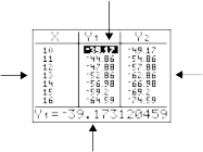
Independent-variable values in the first column
Dependent-variable values in the second and third columns
Current cell’s full value
Note: When the table first displays, the message “Press + for DeltaTbl†is on the entry line. This message reminds you that you can press [+] to change DeltaTbl at any time. When you press any key, the message disappears.
Independent and Dependent Variables
The current graphing mode determines which independent and dependent variables are displayed in the table (Chapter 1). In the table above, for example, the independent variable X and the dependent variables Y1 and Y2 are displayed because Func graphing mode is set.
![]()
Graphing Mode
Independent Variable
Dependent Variable
![]()
Func (function) X Y1 through Y9, and Y0
![]()
Par (parametric) T X1T/Y1T through X6T/Y6T
![]()
Pol (polar) Theta r1 through r6
![]()
Seq (sequence) n u(n), v(n), and w(n)
![]()
Clearing the Table from the Home Screen or a Program
From the home screen, select the ClrTable instruction from the CATALOG. To clear the table, press
[ENTER].
From a program, select 9:ClrTable from the PRGM I/O menu or from the CATALOG. The table is cleared upon execution. If IndpntAsk is selected, all independent and dependent variable values on the table are cleared. If DependAsk is selected, all dependent variable values on the table are cleared.
Scrolling Independent-Variable Values
If Indpnt: Auto is selected, you can press [up key] and [down key] in the independent-variable column to display more values. As you scroll the column, the corresponding dependent-variable values also are displayed. All dependent-variable values may not be displayed if Depend: Ask is selected.
Note: You can scroll back from the value entered for TblStart. As you scroll, TblStart is updated automatically to the value shown on the top line of the table. In the example above, TblStart=0 and DeltaTbl=1 generates and displays values of X=0, …, 6; but you can press [up key] to scroll back and display the table for X=-1, …, 5.
Changing Table Settings from the Table View
You can change table settings from the table view by highlighting a value in the table, pressing [+], and entering a new Delta value.
Press [Y=] and then press 1 [ALPHA] [F1] 1 2 [right key] [X, T, theta, n] to enter the function Y1=1/2x.
Press [2nd]
[TABLE]. 
Press [down key] [down key] [down key] to move the cursor to highlight 3, and then press [+].
Press 1 [ALPHA] [F1] 1 2 to change the table settings to view changes in X in increments of 1/2.
Press [ENTER]. 
Displaying Other Dependent Variables
If you have defined more than two dependent variables, the first two selected Y= functions are displayed initially. Press [right key] or [left key] to display dependent variables defined by other selected Y= functions. The independent variable always remains in the left column, except during a trace with parametric graphing mode and G-T split-screen mode set.
Note: To simultaneously display two dependent variables on the table that are not defined as consecutive Y= functions, go to the Y= editor and deselect the Y= functions between the two you want to display. For example, to simultaneously display Y4 and Y7 on the table, go to the Y= editor and deselect Y5 and Y6.
Getting Started is a fast-paced introduction. Read the chapter for details.
![]()
-----
Suppose you want to find the equation of the tangent line at X = - 2 for the function Y=sin(X).
2
Before you begin, press [MODE] and select 4, Radian and Func, if necessary.
Press [Y=] to display the Y= editor. Press
[SIN] [X, T, theta, n] [)] to store sin(X) in Y1.
Press [ZOOM] 7 to select 7:ZTrig, which graphs the equation in the Zoom Trig window.
Press [2nd] [DRAW] 5 to select 5:Tangent(. The tangent instruction is initiated.
Press [2nd] [square root key] 2 [)] [division key] 2.
Press [ENTER]. The tangent line is drawn; the X value and the tangent-line equation are displayed on the graph.
Consider repeating this activity with the mode set to the number of decimal places desired. The first screen shows four decimal places. The second screen shows
the
decimal setting at Float. 
DRAW Menu
To display the DRAW menu, press [2nd] [DRAW]. The TI-84 Plus’s interpretation of these instructions depends on whether you accessed the menu from the home screen or the program editor or directly from a graph.
![]()
DRAW POINTS STO
|
1: |
ClrDraw |
Clears all drawn elements. |
|
2: |
Line( |
Draws a line segment between 2 points. |
|
3: |
Horizontal |
Draws a horizontal line. |
|
4: |
Vertical |
Draws a vertical line. |
|
5: |
Tangent( |
Draws a line segment tangent to a function. |
|
6: |
DrawF |
Draws a function. |
|
7: |
Shade( |
Shades an area between two functions. |
|
8: |
DrawInv |
Draws the inverse of a function. |
|
9: |
Circle( |
Draws a circle. |
|
0: |
Text( |
Draws text on a graph screen. |
|
A: |
Pen |
Activates the free-form drawing tool. |
![]()
Before Drawing on a Graph
The DRAW instructions draw on top of graphs. Therefore, before you use the DRAW instructions, consider whether you want to perform one or more of the following actions.
Change the mode settings on the mode screen.
Change the format settings on the format screen. You can press [2nd] [FORMAT] or use the shortcut on the mode screen to go to the format graph screen.
Enter or edit functions in the Y= editor.
Select or deselect functions in the Y= editor.
Change the window variable values.
Turn stat plots on or off.
Clear existing drawings with ClrDraw.
Note: If you draw on a graph and then perform any of the actions listed above, the graph is replotted without the drawings when you display the graph again. Before you clear drawings, you can store them with StorePic.
Drawing on a Graph
You can use any DRAW menu instructions except DrawInv to draw on Func, Par, Pol, and Seq graphs. DrawInv is valid only in Func graphing. The coordinates for all DRAW instructions are the display’s x-coordinate and y-coordinate values.
You can use most DRAW menu and DRAW POINTS menu instructions to draw directly on a graph, using the cursor to identify the coordinates. You also can execute these instructions from the home screen or from within a program. If a graph is not displayed when you select a DRAW menu instruction, the home screen is displayed.
Clearing Drawings When a Graph Is Displayed
All points, lines, and shading drawn on a graph with DRAW instructions are temporary.
To clear drawings from the currently displayed graph, select 1:ClrDraw from the DRAW menu. The current graph is replotted and displayed with no drawn elements.
Clearing Drawings from the Home Screen or a Program
To clear drawings on a graph from the home screen or a program, begin on a blank line on the home screen or in the program editor. Select 1:ClrDraw from the DRAW menu. The instruction is copied to the cursor location. Press [ENTER].
When ClrDraw is executed, it clears all drawings from the current graph and displays the message Done. When you display the graph again, all drawn points, lines, circles, and shaded areas will be gone.
![]()
Note: Before you clear drawings, you can store them with StorePic.
Drawing a Line Segment Directly on a Graph
To draw a line segment when a graph is displayed, follow these steps.
Select 2:Line( from the DRAW menu.
Place the cursor on the point where you want the line segment to begin, and then press
[ENTER].
Move the cursor to the point where you want the line segment to end. The line is displayed as you move the cursor. Press [ENTER].
To continue drawing line segments, repeat steps 2 and 3. To cancel Line(, press [CLEAR].
Drawing a Line Segment from the Home Screen or a Program
Line( also draws a line segment between the coordinates (X1,Y1) and (X2,Y2). The values may be entered as expressions.
Line(X1,Y1,X2,Y2)
To erase a line segment, enter Line(X1,Y1,X2,Y2,0)
Drawing a Line Directly on a Graph
To draw a horizontal or vertical line when a graph is displayed, follow these steps.
Select 3:Horizontal or 4:Vertical from the DRAW menu. A line is displayed that moves as you move the cursor.
Place the cursor on the y-coordinate (for horizontal lines) or x-coordinate (for vertical lines) through which you want the drawn line to pass.
Press [ENTER] to draw the line on the graph.
To continue drawing lines, repeat steps 2 and 3. To cancel Horizontal or Vertical, press [CLEAR].
Drawing a Line from the Home Screen or a Program
Horizontal (horizontal line) draws a horizontal line at Y=y, y, which can be an expression but not a list.
Horizontal y
Vertical (vertical line) draws a vertical line at X=x, x, which can be an expression but not a list.
Vertical x
To instruct the TI-84 Plus to draw more than one horizontal or vertical line, separate each instruction with a colon ( : ).
MathPrintâ„¢ Classic

Drawing a Tangent Line Directly on a Graph
To draw a tangent line when a graph is displayed, follow these steps.
Select 5:Tangent( from the DRAW menu.
Press [down key] and [up key] to move the cursor to the function for which you want to draw the tangent line. The current graph’s Y= function is displayed in the top-left corner, if ExprOn is selected.
Press [right key] and [left key] or enter a number to select the point on the function at which you want to draw the tangent line.
Press [ENTER]. In Func mode, the X value at which the tangent line was drawn is displayed on the bottom of the screen, along with the equation of the tangent line. In all other modes, the dy/dx value is displayed.
Change the fixed decimal setting on the mode screen if you want to see fewer digits displayed for X and the equation for Y.
Drawing a Tangent Line from the Home Screen or a Program
Tangent( (tangent line) draws a line tangent to expression in terms of X, such as Y1 or X squared, at point X=value. X can be an expression. expression is interpreted as being in Func mode.
Tangent(expression,value)
Drawing a Function
DrawF (draw function) draws expression as a function in terms of X on the current graph. When you select 6:DrawF from the DRAW menu, the TI-84 Plus returns to the home screen or the program editor. DrawF is not interactive.
DrawF expression
Note: You cannot use a list in expression to draw a family of curves.
Drawing an Inverse of a Function
DrawInv (draw inverse) draws the inverse of expression by plotting X values on the y-axis and Y values on the x-axis. When you select 8:DrawInv from the DRAW menu, the TI-84 Plus returns to the home screen or the program editor. DrawInv is not interactive. DrawInv works in Func mode only.
DrawInv expression
Note: You cannot use a list of expressions with DrawInv.
Shading a Graph
To shade an area on a graph, select 7:Shade( from the DRAW menu. The instruction is pasted to the home screen or to the program editor.
Shade(lowerfunc,upperfunc[,Xleft,Xright,pattern,patres])
MathPrintâ„¢ Classic
Shade( draws lowerfunc and upperfunc in terms of X on the current graph and shades the area that is specifically above lowerfunc and below upperfunc. Only the areas where lowerfunc < upperfunc are shaded.
Xleft and Xright, if included, specify left and right boundaries for the shading. Xleft and Xright must be numbers between Xmin and Xmax, which are the defaults.
pattern specifies one of four shading patterns.
pattern=1 pattern=2 pattern=3 pattern=4
vertical (default) horizontal negative—slope 45°
positive—slope 45°
patres specifies one of eight shading resolutions.
patres=1 patres=2 patres=3 patres=4 patres=5 patres=6 patres=7 patres=8
shades every pixel (default) shades every second pixel shades every third pixel shades every fourth pixel shades every fifth pixel shades every sixth pixel shades every seventh pixel shades every eighth pixel
Drawing a Circle Directly on a Graph
To draw a circle directly on a displayed graph using the cursor, follow these steps.
Select 9:Circle( from the DRAW menu.
Place the cursor at the center of the circle you want to draw. Press [ENTER].
Move the cursor to a point on the circumference. Press [ENTER] to draw the circle on the graph.
Note: This circle is displayed as circular, regardless of the window variable values, because you drew it directly on the display. When you use the Circle( instruction from the home screen or a program, the current window variables may distort the shape.
To continue drawing circles, repeat steps 2 and 3. To cancel Circle(, press [CLEAR].
Drawing a Circle from the Home Screen or a Program
Circle( draws a circle with center (X,Y) and radius. These values can be expressions.
Circle(X,Y,radius)
Note: When you use Circle( on the home screen or from a program, the current window values may distort the drawn circle. Use ZSquare (Chapter 3) before drawing the circle to adjust the window variables and make the circle circular.
Placing Text Directly on a Graph
To place text on a graph when the graph is displayed, follow these steps.
Select 0:Text( from the DRAW menu.
Place the cursor where you want the text to begin.
Enter the characters. Press [ALPHA] or [2nd] [A-LOCK] to enter letters and theta. You may enter TI-84 Plus functions, variables, and instructions. The font is proportional, so the exact number of characters you can place on the graph varies. As you type, the characters are placed on top of the graph.
To cancel Text(, press [CLEAR].
Placing Text on a Graph from the Home Screen or a Program
Text( places on the current graph the characters comprising value, which can include TI-84 Plus functions and instructions. The top-left corner of the first character is at pixel (row,column), where row is an integer between 0 and 57 and column is an integer between 0 and 94. Both row and column can be expressions.
Text(row,column,value,value…)
value can be text enclosed in quotation marks ( " ), or it can be an expression. The TI-84 Plus will evaluate an expression and display the result with up to 10 characters.
Classic
Split Screen
On a Horiz split screen, the maximum value for row is 25. On a G-T split screen, the maximum value for row is 45, and the maximum value for column is 46.
Using Pen to Draw on a Graph
Pen draws directly on a graph only. You cannot execute Pen from the home screen or a program. You can capture the image you created using TI-Connectâ„¢ software and save it to your computer for homework or teaching material or store it as a picture file on your TI-84 Plus (see Storing Graph Pictures below).
To draw on a displayed graph, follow these steps.
Select A:Pen from the DRAW menu.
Place the cursor on the point where you want to begin drawing. Press [ENTER] to turn on the pen.
Move the cursor. As you move the cursor, you draw on the graph, shading one pixel at a time.
Press [ENTER] to turn off the pen.
For example, Pen was used to create the arrow pointing to the local minimum of the selected function.
Note: To continue drawing on the graph, move the cursor to a new position where you want to begin drawing again, and then repeat steps 2, 3, and 4. To cancel Pen, press [CLEAR].
DRAW POINTS Menu
To display the DRAW POINTS menu, press [2nd] [DRAW] [right key]. The TI-84 Plus’s interpretation of these instructions depends on whether you accessed this menu from the home screen or the program editor or directly from a graph.
![]()
DRAW POINTS STO
|
1: |
Pt-On( |
Turns on a point. |
|
2: |
Pt-Off( |
Turns off a point. |
|
3: |
Pt-Change( |
Toggles a point on or off. |
|
4: |
Pxl-On( |
Turns on a pixel. |
|
5: |
Pxl-Off( |
Turns off a pixel. |
|
6: |
Pxl-Change( |
Toggles a pixel on or off. |
|
7: |
pxl-Test( |
Returns 1 if pixel on, 0 if pixel off. |
![]()
Drawing Points Directly on a Graph with Pt-On(
To draw a point on a graph, follow these steps.
Select 1:Pt-On( from the DRAW POINTS menu.
Move the cursor to the position where you want to draw the point.
Press [ENTER] to draw the point.
To continue drawing points, repeat steps 2 and 3. To cancel Pt-On(, press [CLEAR].
Erasing Points with Pt-Off(
To erase (turn off) a drawn point on a graph, follow these steps.
Select 2:Pt-Off( (point off) from the DRAW POINTS menu.
Move the cursor to the point you want to erase.
Press [ENTER] to erase the point.
To continue erasing points, repeat steps 2 and 3. To cancel Pt-Off(, press [CLEAR].
Changing Points with Pt-Change(
To change (toggle on or off) a point on a graph, follow these steps.
Select 3:Pt-Change( (point change) from the DRAW POINTS menu.
Move the cursor to the point you want to change.
Press [ENTER] to change the point’s on/off status.
To continue changing points, repeat steps 2 and 3. To cancel Pt-Change(, press [CLEAR].
Drawing Points from the Home Screen or a Program
Pt-On( (point on) turns on the point at (X=x,Y=y). Pt-Off( turns the point off. Pt-Change( toggles the point on or off. mark is optional; it determines the point’s appearance; specify 1, 2, or 3, where:
1 = dot; default 2 = box 3 = + cross
Pt-On(x,y[,mark])
Pt-Off(x,y[,mark]) Pt-Change(x,y)
Note: If you specified mark to turn on a point with Pt-On(, you must specify mark when you turn off the point with Pt-Off(. Pt-Change( does not have the mark option.
TI-84 Plus Pixels
A pixel is a square dot on the TI-84 Plus display. The Pxl- (pixel) instructions let you turn on, turn off, or reverse a pixel (dot) on the graph using the cursor. When you select a pixel instruction from
the DRAW POINTS menu, the TI-84 Plus returns to the home screen or the program editor. The pixel instructions are not interactive.
Turning On and Off Pixels with Pxl-On( and Pxl-Off(
Pxl-On( (pixel on) turns on the pixel at (row,column), where row is an integer between 0 and 62 and
column is an integer between 0 and 94.
Pxl-Off( turns the pixel off. Pxl-Change( toggles the pixel on and off.
Pxl-On(row,column) Pxl-Off(row,column) Pxl-Change(row,column)
Using pxl-Test(
pxl-Test( (pixel test) returns 1 if the pixel at (row,column) is turned on or 0 if the pixel is turned off on the current graph. row must be an integer between 0 and 62. column must be an integer between 0 and 94.
pxl-Test(row,column)
Split Screen
On a Horiz split screen, the maximum value for row is 30 for Pxl-On(, Pxl-Off(, Pxl-Change(, and
pxl-Test(.
On a G-T split screen, the maximum value for row is 50 and the maximum value for column is 46 for
Pxl-On(, Pxl-Off(, Pxl-Change(, and pxl-Test(.
DRAW STO Menu
To display the DRAW STO menu, press [2nd] [DRAW] [left key]. When you select an instruction from the DRAW STO menu, the TI-84 Plus returns to the home screen or the program editor. The picture and graph database instructions are not interactive.
![]()
DRAW POINTS STO
|
1: |
StorePic |
Stores the current picture. |
|
2: |
RecallPic |
Recalls a saved picture. |
|
3: |
StoreGDB |
Stores the current graph database. |
|
4: |
RecallGDB |
Recalls a saved graph database. |
![]()
Storing a Graph Picture
You can store up to 10 graph pictures, each of which is an image of the current graph display, in picture variables Pic1 through Pic9, or Pic0. Later, you can superimpose the stored picture onto a displayed graph from the home screen or a program.
A picture includes drawn elements, plotted functions, axes, and tick marks. The picture does not include axes labels, lower and upper bound indicators, prompts, or cursor coordinates. Any parts of the display hidden by these items are stored with the picture.
To store a graph picture, follow these steps.
Select 1:StorePic from the DRAW STO menu. StorePic is pasted to the current cursor location.
Enter the number (from 1 to 9, or 0) of the picture variable to which you want to store the picture. For example, if you enter 3, the TI-84 Plus will store the picture to Pic3.
![]()
Note: You also can select a variable from the PICTURE secondary menu ([VARS] 4). The variable is pasted next to StorePic.
Press [ENTER] to display the current graph and store the picture.
Recalling a Graph Picture
To recall a graph picture, follow these steps.
Select 2:RecallPic from the DRAW STO menu. RecallPic is pasted to the current cursor location.
Enter the number (from 1 to 9, or 0) of the picture variable from which you want to recall a picture. For example, if you enter 3, the TI-84 Plus will recall the picture stored to Pic3.
![]()
Note: You also can select a variable from the PICTURE secondary menu ([VARS] 4). The variable is pasted next to RecallPic.
Press [ENTER] to display the current graph with the picture superimposed on it.
Note: Pictures are drawings. You cannot trace a curve that is part of a picture.
Deleting a Graph Picture
To delete graph pictures from memory, use the MEMORY MANAGEMENT/DELETE secondary menu (Chapter 18).
What Is a Graph Database?
A graph database (GDB) contains the set of elements that defines a particular graph. You can recreate the graph from these elements. You can store up to 10 GDBs in variables GDB1 through GDB9, or GDB0 and recall them to recreate graphs.
A GDB stores five elements of a graph.
Graphing mode
Window variables
Format settings
All functions in the Y= editor and the selection status of each
Graph style for each Y= function
GDBs do not contain drawn items or stat plot definitions.
Storing a Graph Database
To store a graph database, follow these steps.
Select 3:StoreGDB from the DRAW STO menu. StoreGDB is pasted to the current cursor location.
Enter the number (from 1 to 9, or 0) of the GDB variable to which you want to store the graph database. For example, if you enter 7, the TI-84 Plus will store the GDB to GDB7.
![]()
Note: You also can select a variable from the GDB secondary menu ([VARS] 3). The variable is pasted next to StoreGDB.
Press [ENTER] to store the current database to the specified GDB variable.
Recalling a Graph Database
CAUTION: When you recall a GDB, it replaces all existing Y= functions. Consider storing the current Y= functions to another database before recalling a stored GDB.
To recall a graph database, follow these steps.
Select 4:RecallGDB from the DRAW STO menu. RecallGDB is pasted to the current cursor location.
Enter the number (from 1 to 9, or 0) of the GDB variable from which you want to recall a GDB. For example, if you enter 7, the TI-84 Plus will recall the GDB stored to GDB7.
![]()
Note: You also can select a variable from the GDB secondary menu ([VARS] 3). The variable is pasted next to RecallGDB.
Press [ENTER] to replace the current GDB with the recalled GDB. The new graph is not plotted. The TI-84 Plus changes the graphing mode automatically, if necessary.
Deleting a Graph Database
To delete a GDB from memory, use the MEMORY MANAGEMENT/DELETE secondary menu (Chapter 18).
Getting Started is a fast-paced introduction. Read the chapter for details.
Use G-T (graph-table) split-screen mode to explore the unit circle and its relationship to the numeric values for the commonly used trigonometric angles of 0° 30°, 45°, 60°, 90°, and so on.

Press [MODE] to display the mode screen. Press [down key] [down key] [right key] [ENTER] to select Degree mode. Press [down key] [right key] [ENTER] to select Par (parametric) graphing mode.
Press [down key] [down key] [down key] [down key] [right key] [right key] [ENTER] to select G-T (graph- table) split-screen mode.
Press [down key] [down key] [down key] [down key] [right key] [ENTER] to display the format screen. Press [down key] [down key] [down key] [down key] [down key] [right key] [ENTER] to select ExprOff.
Press [Y=] to display the Y= editor for Par graphing mode. Press [COS] [X, T, theta, n] [)] [ENTER] to store cos(T) to X1T. Press [SIN]
[X, T, theta, n] [)] [ENTER] to store sin(T) to Y1T.
Press [WINDOW] to display the window editor.
Enter these values for the window variables.
Tmin=0 Xmin=-2.3 Ymin=-2.5 Tmax=360 Xmax=2.3 Ymax=2.5 Tstep=15 Xscl=1 Yscl=1
Press [TRACE]. On the left, the unit circle is graphed parametrically in Degree mode and the trace cursor is activated. When T=0 (from the graph trace coordinates), you can see from the table on the right that the value of X1T (cos(T)) is 1 and Y1T (sin(T)) is 0. Press [right key] to move the cursor to the next 15° angle increment. As you trace around the circle in steps of 15°, an approximation of the standard value for each angle is highlighted in the table.
Press [2ND] [TBLSET] and change Indpnt to Ask.
Press [2ND] [TABLE] to make the table portion of the split screen active.
Setting a Split-Screen Mode
To set a split-screen mode, press [MODE], and then move the cursor to Horiz or G-T and press
[ENTER].
Select Horiz (horizontal) to display the graph screen and another screen split horizontally.
Select G-T (graph-table) to display the graph screen and table screen split vertically.

The split screen is activated when you press any key that applies to either half of the split screen. If stat plots are turned on, the plots are shown along with the x-y plots in graphs. Press [2ND]
[TABLE] to make the table portion of the split screen active and to display the list data. Press [down key] or [up key] to highlight a value you want to edit, and then enter a new value directly in the table to overwrite the previous value. Press [right key] repeatedly to display each column of data (both table and list data).
Split-screen display with both x-y plots and stat plots
Some screens are never displayed as split screens. For example, if you press [MODE] in Horiz or G-T mode, the mode screen is displayed as a full screen. If you then press a key that displays either half of a split screen, such as [TRACE], the split screen returns.
When you press a key or key combination in either Horiz or G-T mode, the cursor is placed in the half of the display to which that key applies. For example, if you press [TRACE], the cursor is placed in the half where the graph is displayed. If you press [2ND] [TABLE], the cursor is placed in the half where the table is displayed.
The TI-84 Plus will remain in split-screen mode until you change back to Full screen mode.
Horiz Mode
In Horiz (horizontal) split-screen mode, a horizontal line splits the screen into top and bottom halves.

The top half displays the graph.
The bottom half displays any of these screens.
Home screen (four lines)
Y= editor (four lines)
Stat list editor (two rows)
Window editor (three settings)
Table editor (two rows)
Moving from Half to Half in Horiz Mode
To use the top half of the split screen:
Press [GRAPH] or [TRACE].
Select a ZOOM or CALC operation. To use the bottom half of the split screen:
Press any key or key combination that displays the home screen.
Press [Y=] (Y= editor).
Press [STAT] [ENTER] (stat list editor).
Press [WINDOW] (window editor).
Press [2ND] [TABLE] (table editor).
Full Screens in Horiz Mode
All other screens are displayed as full screens in Horiz split-screen mode.
To return to the Horiz split screen from a full screen when in Horiz mode, press any key or key combination that displays the graph, home screen, Y= editor, stat list editor, window editor, or table editor.
G-T Mode
In G-T (graph-table) split-screen mode, a vertical line splits the screen into left and right halves.
The left half displays all active graphs and plots.
The right half displays either table data corresponding to the graph at the left or list data corresponding to the plot at the left.
Moving from Half to Half in G-T Mode
To use the left half of the split screen:
Press [GRAPH] or [TRACE].
Select a ZOOM or CALC operation.
To use the right half of the split screen, press [2ND] [TABLE]. If the values on the right are list data, these values can be edited similarly to using the Stat List Editor.
Using TRACE in G-T Mode
As you press [left key] or [right key] to move the trace cursor along a graph in the split screen’s left half in G-T mode, the table on the right half automatically scrolls to match the current cursor values. If more than one graph or plot is active, you can press [up key] or [down key] to select a different graph or plot.
Note: When you trace in Par graphing mode, both components of an equation (XnT and YnT) are displayed in the two columns of the table. As you trace, the current value of the independent variable T is displayed on the graph.
Full Screens in G-T Mode
All screens other than the graph and the table are displayed as full screens in G-T split-screen mode.
To return to the G-T split screen from a full screen when in G-T mode, press any key or key combination that displays the graph or the table.
TI-84 Plus Pixels in Horiz and G-T Modes
Note: Each set of numbers in parentheses above represents the row and column of a corner pixel, which is turned on.
DRAW POINTS Menu Pixel Instructions
For Pxl-On(, Pxl-Off(, Pxl-Change(, and pxl-Test(:
In Horiz mode, row must be < (less than or equal to) 30; column must be < (less than or equal to) 94.
In G-T mode, row must be < (less than or equal to) 50; column must be < (less than or equal to) 46.
Pxl-On(row,column)
DRAW Menu Text( Instruction
For the Text( instruction:
In Horiz mode, row must be < (less than or equal to) 25; column must be < (less than or equal to) 94.
In G-T mode, row must be < (less than or equal to) 45; column must be < (less than or equal to) 46.
Text(row,column,"text")
PRGM I/O Menu Output( Instruction
For the Output( instruction:
In Horiz mode, row must be < (less than or equal to) 4; column must be < (less than or equal to) 16.
In G-T mode, row must be < (less than or equal to) 8; column must be < (less than or equal to) 16.
Output(row,column,"text")
Note: The Output( instruction can only be used within a program.
Setting a Split-Screen Mode from the Home Screen or a Program
To set Horiz or G-T from a program, follow these steps.
Press [MODE] while the cursor is on a blank line in the program editor.
Select Horiz or G-T.
The instruction is pasted to the cursor location. The mode is set when the instruction is encountered during program execution. It remains in effect after execution.
Note: You also can paste Horiz or G-T to the home screen or program editor from the CATALOG (Chapter 15).
Getting Started is a fast-paced introduction. Read the chapter for details.
You can use the MTRX shortcut menu ([ALPHA] [F3]) to enter a quick matrix calculation on the home screen or in the Y= editor.
Note: To input a fraction in a matrix, delete the pre-populated zero first.
Example: Add the following matrices: ![]() and store the result to matrix C.
and store the result to matrix C.
Press [ALPHA] [F3] to display the quick matrix editor. The default size of the matrix is two rows by two columns.
Press [down key] [down key] to highlight OK and then press [ENTER].
Press 2 [right key] [(-)] 3 [right key] 5 [right key] 8
[right key] to create the first matrix.
Press [+] [ALPHA] [F3] [down key] [down key] [ENTER] 4 [right key] 3 [right key] 2 [right key] 1 [right key] [ENTER] to create the second matrix and perform the calculation.
Press [STO right arrow] [2nd] [MATRX] and select
3:[C].
Press [ENTER] to store the matrix to [C]. 
In the matrix editor ([2nd] [MATRX]), you can see that matrix [C] has dimension 2x2.
You can press [right key] [right key] to display the EDIT
screen and then select [C] to edit it.
Getting Started is a fast-paced introduction. Read the chapter for details.
Find the solution of X + 2Y + 3Z = 3 and 2X + 3Y + 4Z = 3. On the TI-84 Plus, you can solve a system of linear equations by entering the coefficients as elements in a matrix, and then using rref( to obtain the reduced row-echelon form.
Press [2nd] [MATRX]. Press [right key] [right key] to display the MATRX EDIT menu. Press 1 to select 1: [A].
Press 2 [ENTER] 4 [ENTER] to define a 2×4 matrix. The rectangular cursor indicates the current element. Ellipses (...) indicate additional columns beyond the screen.
Press 1 [ENTER] to enter the first element. The rectangular cursor moves to the second column of the first row.
Press 2 [ENTER] 3 [ENTER] 3 [ENTER] to
complete the first row for X + 2Y + 3Z = 3.
Press 2 [ENTER] 3 [ENTER] 4 [ENTER] 3 [ENTER]
to enter the second row for 2X + 3Y + 4Z = 3.
Press [2nd] [QUIT] to return to the home screen. If necessary, press [CLEAR] to clear the home screen. Press [2nd] [MATRX] [right key] to display the MATRX MATH menu. Press [up key] to wrap to the end of the menu. Select B:rref( to copy rref( to the home screen.
Press [2nd] [MATRX] 1 to select 1: [A] from the
MATRX NAMES menu. Press [ ) ] [ENTER]. The
reduced row-echelon form of the matrix is displayed and stored in Ans.
|
1X - 1Z = -3 |
therefore |
X = -3 + Z |
|
1Y + 2Z = 3 |
therefore |
Y = 3 - 2Z |
What Is a Matrix?
A matrix is a two-dimensional array. You can display, define, or edit a matrix in the matrix editor. You can also define a matrix using the MTRX shortcut menu ([ALPHA] [F3]).The TI-84 Plus has 10 matrix variables, [A] through [J]. You can define a matrix directly in an expression. A matrix, depending on available memory, may have up to 99 rows or columns. You can store only real numbers in TI-84 Plus matrices. Fractions are stored as real numbers and can be used in matrices.
Selecting a Matrix
Before you can define or display a matrix in the editor, you first must select the matrix name. To do so, follow these steps.
Press [2nd] [MATRX] [left key] to display the MATRX EDIT menu. The dimensions of any previously defined matrices are displayed.
Select the matrix you want to define. The MATRX EDIT screen is displayed.
![]()
Accepting or Changing Matrix Dimensions
The dimensions of the matrix (row × column) are displayed on the top line. The dimensions of a new matrix are 1 × 1. You must accept or change the dimensions each time you edit a matrix. When you select a matrix to define, the cursor highlights the row dimension.
To accept the row dimension, press [ENTER].
To change the row dimension, enter the number of rows (up to 99), and then press [ENTER].
The cursor moves to the column dimension, which you must accept or change the same way you accepted or changed the row dimension. When you press [ENTER], the rectangular cursor moves to the first matrix element.
Displaying Matrix Elements
After you have set the dimensions of the matrix, you can view the matrix and enter values for the matrix elements. In a new matrix, all values are zero.
Select the matrix from the MATRX EDIT menu and enter or accept the dimensions. The center portion of the matrix editor displays up to seven rows and three columns of a matrix, showing the values of the elements in abbreviated form if necessary. The full value of the current element, which is indicated by the rectangular cursor, is displayed on the bottom line.

This is an 8 × 4 matrix. Ellipses in the left or right column indicate additional columns. Up arrow or
down arrow in the right column indicate additional rows.
Deleting a Matrix
To delete matrices from memory, use the MEMORY MANAGEMENT/DELETE secondary menu (Chapter 18).
Viewing a Matrix
The matrix editor has two contexts, viewing and editing. In viewing context, you can use the cursor keys to move quickly from one matrix element to the next. The full value of the highlighted element is displayed on the edit line.
Select the matrix from the MATRX EDIT menu, and then enter or accept the dimensions.
Using Viewing-Context Keys
![]()
![]()
Key Function
[left key] or [right key]
![]()
[down key] or [up key]
Moves the cursor within the current row
Moves the cursor within the current column; on the top row, [up key] moves the cursor to the column dimension; on the column dimension, [up key] moves the cursor to the row dimension
![]()
[ENTER] Switches to editing context; activates the edit cursor on the bottom line
![]()
![]()
[CLEAR] Switches to editing context; clears the value on the bottom line Any entry character Switches to editing context; clears the value on the bottom line;
copies the character to the bottom line
![]()
[2nd] [INS] Nothing
![]()
[DEL] Nothing
![]()
Editing a Matrix Element
In editing context, an edit cursor is active on the bottom line. To edit a matrix element value, follow these steps.
Select the matrix from the MATRX EDIT menu, and then enter or accept the dimensions.
Press [left key], [up key], [right key], and [down key] to move the cursor to the matrix element you want to change.
Switch to editing context by pressing [ENTER], [CLEAR], or an entry key.
Change the value of the matrix element using the editing-context keys described below. You may enter an expression, which is evaluated when you leave editing context.
Note: You can press [CLEAR] [ENTER] to restore the value at the cursor if you make a mistake.
Press [ENTER], [up key], or [down key] to move to another element.
Using Editing-Context Keys
![]()
Key Function
![]()
|[left key] or [right key] Moves the edit cursor within the value
![]()
[down key] or [up key] Stores the value displayed on the edit line to the matrix element; switches to viewing context and moves the cursor within the column
![]()
[ENTER] Stores the value displayed on the edit line to the matrix element; switches to viewing context and moves the cursor to the next row element
![]()
[CLEAR] Clears the value on the bottom line
![]()
Any entry character Copies the character to the location of the edit cursor on the bottom line
![]()
[2nd] [INS] Activates the insert cursor
![]()
[DEL] Deletes the character under the edit cursor on the bottom line
![]()
To use a matrix in an expression, you can do any of the following.
Copy the name from the MATRX NAMES menu.
Recall the contents of the matrix into the expression with [2nd] [RCL] (Chapter 1).
Enter the matrix directly (see below).
Entering a Matrix in an Expression
You can enter, edit, and store a matrix in the matrix editor. You also can enter a matrix directly in an expression.
To enter a matrix in an expression, follow these steps.
Press [2nd] [ [ ] to indicate the beginning of the matrix.
Press [2nd] [ [ ] to indicate the beginning of a row.
Enter a value, which can be an expression, for each element in the row. Separate the values with commas.
Press [2nd] [ ] ] to indicate the end of a row.
Repeat steps 2 through 4 to enter all of the rows.
Press [2nd] [ ] ] to indicate the end of the matrix.
The resulting matrix is displayed in the form:
[[element1,1,...,element1,n],...,[elementm,1,...,elementm,n]]
Any expressions are evaluated when the entry is executed.
![]()
Note:
The commas that you must enter to separate elements are not displayed on output.
Closing brackets are required when you enter a matrix directly on the home screen or in an expression.
When you define a matrix using the matrix editor, it is automatically stored. However, when you enter a matrix directly on the home screen or in an expression, it is not automatically stored, but you can store it.
In MathPrintâ„¢ mode, you could also use the MTRX shortcut menu to enter this kind of matrix:
Press [ALPHA] [F3] [down key] [right key] [right key] [ENTER] [down key] [ENTER] to define the matrix dimension.
Press 1 [right key] 2 [right key] 2 [right key] 4 [right key] 5 [right key] 6 [right key] to define the matrix.
Press [ENTER] to perform the calculation.
Displaying a Matrix
To display the contents of a matrix on the home screen, select the matrix from the MATRX NAMES
menu, and then press [ENTER].
In MathPrintâ„¢ mode:
An arrow at the left or right indicates additional columns.
An arrow at the top or bottom indicates additional rows. In Classic mode:
Ellipses in the left or right column indicate additional columns.
up arrow or down arrow in the right column indicate additional rows.
In either mode, press [right key], [left key], [down key], and [up key] to scroll the matrix. You can scroll the matrix after you press [ENTER] to calculate the matrix. If you cannot scroll the matrix, press [up key] [ENTER] [ENTER] to repeat the calculation.
MathPrintâ„¢ Classic
Note:
You cannot copy a matrix output from the history.
Matrix calculations are not saved when you change from MathPrintâ„¢ mode to Classic mode or vice-versa.
Copying One Matrix to Another
To copy a matrix, follow these steps.
Press [2nd] [MATRIX] to display the MATRX NAMES menu.
Select the name of the matrix you want to copy.
Press [STO right arrow].
Press [2nd] [MATRIX] again and select the name of the new matrix to which you want to copy the existing matrix.
Press [ENTER] to copy the matrix to the new matrix name.
Accessing a Matrix Element
On the home screen or from within a program, you can store a value to, or recall a value from, a matrix element. The element must be within the currently defined matrix dimensions. Select matrix from the MATRX NAMES menu.
[matrix](row,column)
Using Math Functions with Matrices
You can use many of the math functions on the TI-84 Plus keypad, the MATH menu, the MATH NUM menu, and the MATH TEST menu with matrices. However, the dimensions must be appropriate. Each of the functions below creates a new matrix; the original matrix remains the same.
Addition, Subtraction, Multiplication
To add or subtract matrices, the dimensions must be the same. The answer is a matrix in which the elements are the sum or difference of the individual corresponding elements.
matrixA+matrixB matrixA-matrixB
To multiply two matrices together, the column dimension of matrixA must match the row dimension of matrixB.
matrixA*matrixB
Multiplying a matrix by a value or a value by a matrix returns a matrix in which each element of matrix
is multiplied by value.
matrix*value value*matrix
Negation
Negating a matrix returns a matrix in which the sign of every element is changed.
-matrix
abs(
abs( (absolute value, MATH NUM menu) returns a matrix containing the absolute value of each element of matrix.
abs(matrix)
round(
round( (MATH NUM menu) returns a matrix. It rounds every element in matrix to #decimals (< (less than or equal to) 9). If #decimals is omitted, the elements are rounded to 10 digits.
round(matrix[,#decimals])
Inverse
Use the superscript -1 function ([x superscript -1]) or [^] -1 to invert a matrix. matrice must be square. The determinant cannot equal zero.
-1
![]()
matrix to the
![]()
Powers
To raise a matrix to a power, matrix must be square. You can use square ([x square]), cube (MATH menu), or ^power ([^]) for integer power between 0 and 255.
matrix square matrix cube matrix^power
MathPrintâ„¢
Classic
Relational Operations
To compare two matrices using the relational operations = and does not equal (TEST menu), they must have the same dimensions. = and does not equal compare matrixA and matrixB on an element- by-element basis. The other relational operations are not valid with matrices.
matrixA=matrixB returns 1 if every comparison is true; it returns 0 if any comparison is false.
matrixA does not equal matrixB returns 1 if at least one comparison is false; it returns 0 if no comparison is false.
iPart(, fPart(, int(
iPart( (integer part), fPart( (fractional part), and int( (greatest integer) are on the MATH NUM menu.
iPart( returns a matrix containing the integer part of each element of matrix. fPart( returns a matrix containing the fractional part of each element of matrix. int( returns a matrix containing the greatest integer of each element of matrix.
iPart(matrix) fPart(matrix) int(matrix)
![]()
MATRX MATH Menu
To display the MATRX MATH menu, press [2nd] [MATRX] [right key].
![]()
![]()
NAMES MATH EDIT
|
1: |
det( |
Calculates the determinant. |
|
2: |
superscript T |
Transposes the matrix. |
|
3: |
dim( |
Returns the matrix dimensions. |
|
4: |
Fill( |
Fills all elements with a constant. |
|
5: |
identity( |
Returns the identity matrix. |
|
6: |
randM( |
Returns a random matrix. |
|
7: |
augment( |
Appends two matrices. |
|
8: |
Matrâ–ºlist( |
Stores a matrix to a list. |
![]()
NAMES MATH EDIT
9: Listâ–ºmatr( Stores a list to a matrix.
0: cumSum( Returns the cumulative sums of a matrix.
A: ref( Returns the row-echelon form of a matrix.
B: rref( Returns the reduced row-echelon form.
C: rowSwap( Swaps two rows of a matrix.
D: row+( Adds two rows; stores in the second row.
E: *row( Multiplies the row by a number.
F: *row+( Multiplies the row, adds to the second row.
![]()
det(
det( (determinant) returns the determinant (a real number) of a square matrix.
det(matrix)
Transpose
superscript T (transpose) returns a matrix in which each element (row, column) is swapped with the corresponding element (column, row) of matrix.
matrix superscriptT
Accessing Matrix Dimensions with dim(
dim( (dimension) returns a list containing the dimensions ({rows columns}) of matrix.
dim(matrix)
Note: dim(matrix) right arrow Ln:Ln(1) returns the number of rows. dim(matrix) right arrow Ln:Ln(2)
returns the number of columns.
Creating a Matrix with dim(
Use dim( with [STO right arrow] to create a new matrixname of dimensions rows × columns with 0 as each element.
{rows,columns}right arrow dim(matrixname)
Redimensioning a Matrix with dim(
Use dim( with [STO right arrow] to redimension an existing matrixname to dimensions rows × columns. The elements in the old matrixname that are within the new dimensions are not changed. Additional created elements are zeros. Matrix elements that are outside the new dimensions are deleted.
{rows,columns} right arrow dim(matrixname)
Fill(
Fill( stores value to every element in matrixname.
Fill(value,matrixname)
identity(
identity( returns the identity matrix of dimension rows × dimension columns.
identity(dimension)
randM(
randM( (create random matrix) returns a rows × columns random matrix of integers > (greater than or equal to) -9 and < (less than or equal to) 9. The seed value stored to the rand function controls the values (Chapter 2).
randM(rows,columns)
augment(
augment( appends matrixA to matrixB as new columns. matrixA and matrixB both must have the same number of rows.
augment(matrixA,matrixB)
Matrâ–ºlist(
Matrâ–ºlist( (matrix stored to list) fills each listname with elements from each column in matrix.
Matrâ–ºlist( ignores extra listname arguments. Likewise, Matrâ–ºlist( ignores extra matrix columns.
Matrâ–ºlist(matrix,listnameA,...,listname n)
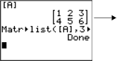
Matrâ–ºlist( also fills a listname with elements from a specified column# in matrix. To fill a list with a specific column from matrix, you must enter column# after matrix.
Matrâ–ºlist(matrix,column#,listname)
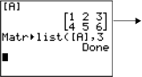
Listâ–ºmatr(
Listâ–ºmatr( (lists stored to matrix) fills matrixname column by column with the elements from each list. If dimensions of all lists are not equal, Listâ–ºmatr( fills each extra matrixname row with 0. Complex lists are not valid.
Listâ–ºmatr(listA,...,list n,matrixname)
![]()
cumSum(
cumSum( returns cumulative sums of the elements in matrix, starting with the first element. Each element is the cumulative sum of the column from top to bottom.
cumSum(matrix)
Row Operations
MATRX MATH menu items A through F are row operations. You can use a row operation in an expression. Row operations do not change matrix in memory. You can enter all row numbers and values as expressions. You can select the matrix from the MATRX NAMES menu.
ref(, rref(
ref( (row-echelon form) returns the row-echelon form of a real matrix. The number of columns must be greater than or equal to the number of rows.
ref(matrix)
rref( (reduced row-echelon form) returns the reduced row-echelon form of a real matrix. The number of columns must be greater than or equal to the number of rows.
rref(matrix)
rowSwap(
rowSwap( returns a matrix. It swaps rowA and rowB of matrix.
rowSwap(matrix,rowA,rowB)
row+(
row+( (row addition) returns a matrix. It adds rowA and rowB of matrix and stores the results in rowB.
row+(matrix,rowA,rowB)
*row(
*row( (row multiplication) returns a matrix. It multiplies row of matrix by value and stores the results in row.
*row(value,matrix,row)
*row+(
*row+( (row multiplication and addition) returns a matrix. It multiplies rowA of matrix by value, adds it to rowB, and stores the results in rowB.
*row+(value,matrix,rowA,rowB)
Getting Started is a fast-paced introduction. Read the chapter for details.
Calculate the first eight terms of the sequence 1/A square. Store the results to a user-created list. Then display the results in fraction form. Begin this example on a blank line on the home screen.
Press [2nd] [LIST] [right key] to display the
LIST OPS menu.
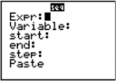
Press 5 to select 5:seq(, which opens a wizard to assist in the entry of the syntax.
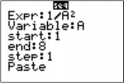
Press 1 [ALPHA] [F1] [ENTER] [ALPHA] [A] [x
square] [down key] [ALPHA] [A] [down key] 1 [down key] 8 [down key] 1 to enter the sequence.
Press [down key], to select Paste, and press [ENTER] to paste the seq( to the current cursor location.
Press [STO right arrow], and then press [2nd] [A- LOCK] to turn on alpha-lock. Press [S] [E] [Q], and then press [ALPHA] to turn off alpha-lock. Press 1 to complete the list name.
Note: Since the seq( command creates a list, you can name give the list a name up to five characters long.
Press [ENTER] to generate the list and store it in SEQ1. The list is displayed on the home screen. An ellipsis (...) indicates that the list continues beyond the viewing window. Press [right key] repeatedly (or press and hold [right key]) to scroll the list and view all the list elements.
Press [2nd] [LIST] to display the LIST NAMES menu. Press 7 to select 7:SEQ1 to paste LSEQ1 to the current cursor location. (If SEQ1 is not item 7 on your LIST NAMES menu, move the cursor to SEQ1 before you press [ENTER].)
Press [MATH] to display the MATH menu. Press 2 to select 2:4Dec, which pastes right triangleDec to the current cursor location.
Press [ENTER] to show the sequence in decimal form. Press [right key] repeatedly (or press and hold [right key]) to scroll the list and view all the list elements.
Using TI-84 Plus List Names L1 through L6
The TI-84 Plus has six list names in memory: L1, L2, L3, L4, L5, and L6. The list names L1 through L6 are the second functions of [1] through [6]. To paste one of these names to a valid screen, press [2nd], and then press the appropriate key. L1 through L6 are stored in stat list editor columns 1 through 6 when you reset memory.
Creating a List Name on the Home Screen
To create a list name on the home screen, follow these steps.
Press [2nd] [{], enter one or more list elements, and then press [2nd] [}]. Separate list elements with commas. List elements can be real numbers, complex numbers, or expressions.
![]()
Press [STO right arrow].
Press [ALPHA] [letter from A to Z or theta] to enter the first letter of the name.
Enter zero to four letters, theta, or numbers to complete the name.
![]()
Press [ENTER]. The list is displayed on the next line. The list name and its elements are stored in memory. The list name becomes an item on the LIST NAMES menu.
![]()
![]()
Note: If you want to view a user-created list in the stat list editor, you must retrieve the list in the stat list editor (Chapter 12).
You also can create a list name in these four places.
At the Name= prompt in the stat list editor
At an Xlist:, Ylist:, or Data List: prompt in the stat plot editor
At a List:, List1:, List2:, Freq:, Freq1:, Freq2:, XList:, or YList: prompt in the inferential stat editors
On the home screen using SetUpEditor
You can create as many list names as your TI-84 Plus memory has space to store.
Storing Elements to a List
You can store list elements in either of two ways.
Use brackets and [STO right arrow] on the home screen.
![]()
Use the stat list editor (Chapter 12).
The maximum dimension of a list is 999 elements.
Note: When you store a complex number to a list, the entire list is converted to a list of complex numbers. To convert the list to a list of real numbers, display the home screen, and then enter real(listname) right arrow listname.
Displaying a List on the Home Screen
To display the elements of a list on the home screen, enter the name of the list (preceded by L, if necessary), and then press [ENTER]. An ellipsis indicates that the list continues beyond the viewing window. Press [right key] repeatedly (or press and hold [right key]) to scroll the list and view all the list elements.
![]()
Copying One List to Another
To copy a list, store it to another list.
![]()
Accessing a List Element
You can store a value to or recall a value from a specific list element. You can store to any element within the current list dimension or one element beyond.
listname(element)
Deleting a List from Memory
To delete lists from memory, including L1 through L6, use the MEMORY MANAGEMENT/DELETE secondary menu (Chapter 18). Resetting memory restores L1 through L6. Removing a list from the stat list editor does not delete it from memory.
Using Lists in Graphing
To graph a family of curves, you can use lists (Chapter 3) or the Transformation Graphing App.
Using the LIST NAMES Menu
To display the LIST NAMES menu, press [2nd] [LIST]. Each item is a user-created list name except for L1 through L6. LIST NAMES menu items are sorted automatically in alphanumerical order. Only the first 10 items are labeled, using 1 through 9, then 0. To jump to the first list name that begins with a particular alpha character or theta, press [ALPHA] [letter from A to Z or theta].
![]()
Note: From the top of a menu, press [up key] to move to the bottom. From the bottom, press [down key] to move to the top.
When you select a list name from the LIST NAMES menu, the list name is pasted to the current cursor location.
The list name symbol L precedes a list name when the name is pasted where non-list name data also is valid, such as the home screen.
![]()
The L symbol does not precede a list name when the name is pasted where a list name is the only valid input, such as the stat list editor’s Name= prompt or the stat plot editor’s XList: and YList: prompts.
Entering a User-Created List Name Directly
To enter an existing list name directly, follow these steps.
Press [2nd] [LIST] [right key] to display the LIST OPS menu.
Select B: L, which pastes L the current cursor location. L is not always necessary.
Note: You also can paste L to the current cursor location from the CATALOG.
Enter the characters that comprise the list name.
![]()
Attaching a Formula to a List Name
You can attach a formula to a list name so that each list element is a result of the formula. When executed, the attached formula must resolve to a list.
When anything in the attached formula changes, the list to which the formula is attached is updated automatically.
When you edit an element of a list that is referenced in the formula, the corresponding element in the list to which the formula is attached is updated.
When you edit the formula itself, all elements in the list to which the formula is attached are updated.
For example, the first screen below shows that elements are stored to L3, and the formula L3+10 is attached to the list name LADD10. The quotation marks designate the formula to be attached to LADD10. Each element of LADD10 is the sum of an element in L3 and 10.
The next screen shows another list, L4. The elements of L4 are the sum of the same formula that is attached to L3. However, quotation marks are not entered, so the formula is not attached to L4.
On the next line, -6 right arrow L3(1):L3 changes the first element in L3 to -6, and then redisplays
L3.
![]()
The last screen shows that editing L3 updated LADD10, but did not change L4. This is because the formula L3+10 is attached to LADD10, but it is not attached to L4.
![]()
Note: To view a formula that is attached to a list name, use the stat list editor (Chapter 12).
Attaching a Formula to a List on the Home Screen or in a Program
To attach a formula to a list name from a blank line on the home screen or from a program, follow these steps.
Press [ALPHA] ["], enter the formula (which must resolve to a list), and press [ALPHA] ["]
again.
Note: When you include more than one list name in a formula, each list must have the same dimension.
Press [STO right arrow].
Enter the name of the list to which you want to attach the formula.
Press [2nd], and then enter a TI-84 Plus list name L1 through L6.
Press [2nd] [LIST] and select a user-created list name from the LIST NAMES menu.
Enter a user-created list name directly using L.
Press [ENTER].
Note: The stat list editor displays a formula-lock symbol next to each list name that has an attached formula. Chapter 12 describes how to use the stat list editor to attach formulas to lists, edit attached formulas, and detach formulas from lists.
Detaching a Formula from a List
You can detach (clear) an attached formula from a list in several ways. For example:
Enter " " right arrow listname on the home screen.
Edit any element of a list to which a formula is attached.
Use the stat list editor (Chapter 12).
Use ClrList or ClrAllList to detach a formula from a list (Chapter 18).
You can use lists in an expression in any of three ways. When you press [ENTER], any expression is evaluated for each list element, and a list is displayed.
Use L1–L6 or any user-created list name in an expression.
![]()
Enter the list elements directly.
![]()
Use [2nd] [RCL] to recall the contents of the list into an expression at the cursor location (Chapter 1).
![]()
![]()
Note: You must paste user-created list names to the Rcl prompt by selecting them from the
LIST NAMES menu. You cannot enter them directly using L.
Using Lists with Math Functions
You can use a list to input several values for some math functions. See Appendix A specify for information about where a list is valid. The function is evaluated for each list element, and a list is displayed.
When you use a list with a function, the function must be valid for every element in the list. In graphing, an invalid element, such as -1 in square root of ({1,0,-1}), is ignored.
![]() This returns an error.
This returns an error.
![]()
This graphs X*square root of (1) and X*square root of (0), but skips X*square root of (-1).
When you use two lists with a two-argument function, the dimension of each list must be the same. The function is evaluated for corresponding elements.
![]()
When you use a list and a value with a two-argument function, the value is used with each element in the list.
![]()
LIST OPS Menu
To display the LIST OPS menu, press [2nd] [LIST] [right key].
![]()
NAMES OPS MATH
|
1: |
SortA( |
Sorts lists in ascending order. |
|
2: |
SortD( |
Sorts lists in descending order. |
|
3: |
dim( |
Sets the list dimension. |
|
4: |
Fill( |
Fills all elements with a constant. |
|
5: |
seq( |
Creates a sequence. |
|
6: |
cumSum( |
Returns a list of cumulative sums. |
|
7: |
DeltaList( |
Returns difference of successive elements. |
|
8: |
Select( |
Selects specific data points. |
|
9: |
augment( |
Concatenates two lists. |
|
0: |
Listâ–ºmatr( |
Stores a list to a matrix. |
|
A: |
Matrâ–ºlist( |
Stores a matrix to a list. |
|
B: |
L |
Designates the list-name data type. |
![]()
SortA(, SortD(
SortA( (sort ascending) sorts list elements from low to high values. SortD( (sort descending) sorts list elements from high to low values. Complex lists are sorted based on magnitude (modulus).
With one list, SortA( and SortD( sort the elements of listname and update the list in memory.
SortA(listname) SortD(listname)
With two or more lists, SortA( and SortD( sort keylistname, and then sort each dependlist by placing its elements in the same order as the corresponding elements in keylistname. All lists must have the same dimension.
SortA(keylistname,dependlist1[,dependlist2, ...,dependlist n]) SortD(keylistname,dependlist1[,dependlist2, ...,dependlist n])
Note:
In the example, 5 is the first element in L4, and 1 is the first element in L5. After SortA(L4,L5), 5 becomes the second element of L4, and likewise, 1 becomes the second element of L5.
SortA( and SortD( are the same as SortA( and SortD( on the STAT EDIT menu (Chapter 12).
You cannot sort a locked list.
Using dim( to Find List Dimensions
dim( (dimension) returns the length (number of elements) of list.
dim(list)
![]()
Using dim( to Create a List
You can use dim( with [STO right arrow] to create a new listname with dimension length from 1 to 999. The elements are zeros.
length right arrow dim(listname)
![]()
Using dim( to Redimension a List
You can use dim with [STO right arrow] to redimension an existing listname to dimension length from 1 to 999.
The elements in the old listname that are within the new dimension are not changed.
Extra list elements are filled by 0.
Elements in the old list that are outside the new dimension are deleted.
length right arrow dim(listname)
Fill(
Fill( replaces each element in listname with value.
Fill(value,listname)
Note: dim( and Fill( are the same as dim( and Fill( on the MATRX MATH menu (Chapter 10).
seq(
seq( (sequence) returns a list in which each element is the result of the evaluation of expression with regard to variable for the values ranging from begin to end at steps of increment. variable need not be defined in memory. increment can be negative; the default value for increment is 1. seq( is not valid within expression. Complex lists are not valid.
A wizard will open to assist the entry of the syntax.
Note: seq( is the only function in LIST OPS that has a wizard.
seq(expression,variable,begin,end[,increment])
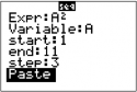
![]()
cumSum(
cumSum( (cumulative sum) returns the cumulative sums of the elements in list, starting with the first element. list elements can be real or complex numbers.
cumSum(list)
![]()
Delta List(
DeltaList( returns a list containing the differences between consecutive elements in list. DeltaList subtracts the first element in list from the second element, subtracts the second element from the third, and so on. The list of differences is always one element shorter than the original list. list elements can be a real or complex numbers.
DeltaList(list)
Select(
Select( selects one or more specific data points from a scatter plot or xyLine plot (only), and then stores the selected data points to two new lists, xlistname and ylistname. For example, you can use Select( to select and then analyze a portion of plotted CBL 2â„¢/CBLâ„¢ or CBRâ„¢ data.
Select(xlistname,ylistname)
Note: Before you use Select(, you must have selected (turned on) a scatter plot or xyLine plot. Also, the plot must be displayed in the current viewing window.
Before Using Select(
Before using Select(, follow these steps.
Create two list names and enter the data.
Turn on a stat plot, select scatter plot or xyLine, and enter the two list names for Xlist: and Ylist:
(Chapter 12).
Use ZoomStat to plot the data (Chapter 3).
MathPrintâ„¢
Classic
Using Select( to Select Data Points from a Plot
To select data points from a scatter plot or xyLine plot, follow these steps.
Press [2nd] [LIST] [right key] 8 to select 8:Select( from the LIST OPS menu. Select( is pasted to the home screen.
Enter xlistname, press [,], enter ylistname, and then press [ )] to designate list names into which you want the selected data to be stored.
![]()
Press [ENTER]. The graph screen is displayed with Left Bound? in the bottom-left corner.
Press [up key] or [down key] (if more than one stat plot is selected) to move the cursor onto the stat plot from which you want to select data points.
Press [left key] and [right key] to move the cursor to the stat plot data point that you want as the left bound.
Press [ENTER]. A right triangle indicator on the graph screen shows the left bound. Right Bound? is displayed in the bottom-left corner.
Press [left key] or [right key] to move the cursor to the stat plot point that you want for the right bound, and then press [ENTER].
The x-values and y-values of the selected points are stored in xlistname and ylistname. A new stat plot of xlistname and ylistname replaces the stat plot from which you selected data points. The list names are updated in the stat plot editor.
Note: The two new lists (xlistname and ylistname) will include the points you select as left bound and right bound. Also, left-bound x-value < (less than or equal to) right-bound x-value must be true.
augment(
augment( concatenates the elements of listA and listB. The list elements can be real or complex numbers.
augment(listA,listB)

Listâ–ºmatr(
Listâ–ºmatr( (lists stored to matrix) fills matrixname column by column with the elements from each list. If the dimensions of all lists are not equal, then Listâ–ºmatr( fills each extra matrixname row with
Complex lists are not valid.
Listâ–ºmatr(list1,list2, ... ,list n,matrixname)
![]()

Matrâ–ºlist(
Matrâ–ºlist( (matrix stored to lists) fills each listname with elements from each column in matrix. If the number of listname arguments exceeds the number of columns in matrix, then Matrâ–ºlist( ignores extra listname arguments. Likewise, if the number of columns in matrix exceeds the number of listname arguments, then Matrâ–ºlist( ignores extra matrix columns.
Matrâ–ºlist(matrix,listname1,listname2, . . . ,listname n)
![]()
Matrâ–ºlist( also fills a listname with elements from a specified column# in matrix. To fill a list with a specific column from matrix, you must enter a column# after matrix.
Matrâ–ºlist(matrix,column#,listname)
![]()

L preceding one to five characters identifies those characters as a user-created listname. listname
may comprise letters, theta, and numbers, but it must begin with a letter from A to Z or theta.
Llistname
Generally, L must precede a user-created list name when you enter a user-created list name where other input is valid, for example, on the home screen. Without the L, the TI-84 Plus may misinterpret a user-created list name as implied multiplication of two or more characters.
L need not precede a user-created list name where a list name is the only valid input, for example, at the Name= prompt in the stat list editor or the Xlist: and Ylist: prompts in the stat plot editor. If you enter L where it is not necessary, the TI-84 Plus will ignore the entry.
LIST MATH Menu
To display the LIST MATH menu, press [2nd] [LIST] [left key].
![]()
NAMES OPS MATH
|
1: |
min( |
Returns minimum element of a list. |
|
2: |
max( |
Returns maximum element of a list. |
|
3: |
mean( |
Returns mean of a list. |
|
4: |
median( |
Returns median of a list. |
|
5: |
sum( |
Returns sum of elements in a list. |
|
6: |
prod( |
Returns product of elements in list. |
|
7: |
stdDev( |
Returns standard deviation of a list. |
|
8: |
variance( |
Returns the variance of a list. |
![]()
min(, max(
min( (minimum) and max( (maximum) return the smallest or largest element of listA. If two lists are compared, it returns a list of the smaller or larger of each pair of elements in listA and listB. For a complex list, the element with smallest or largest magnitude (modulus) is returned.
min(listA[,listB]) max(listA[,listB])
MathPrintâ„¢ Classic
Note: min( and max( are the same as min( and max( on the MATH NUM menu.
mean(, median(
mean( returns the mean value of list. median( returns the median value of list. The default value for freqlist is 1. Each freqlist element counts the number of consecutive occurrences of the corresponding element in list. Complex lists are not valid.
mean(list[,freqlist]) median(list[,freqlist])
MathPrintâ„¢ Classic
sum(, prod(
sum( (summation) returns the sum of the elements in list. start and end are optional; they specify a range of elements. list elements can be real or complex numbers.
prod( returns the product of all elements of list. start and end elements are optional; they specify a range of list elements. list elements can be real or complex numbers.
sum(list[,start,end]) prod(list[,start,end])
Sums and Products of Numeric Sequences
You can combine sum( or prod( with seq( to obtain:
upper
G expression(x) x=lower
upper
 expression(x) x=lower
To evaluate Sigma 2 to the (N–1) from N=1 to 4:
![]()
stdDev(, variance(
stdDev( returns the standard deviation of the elements in list. The default value for freqlist is 1. Each freqlist element counts the number of consecutive occurrences of the corresponding element in list. Complex lists are not valid.
stdDev(list[,freqlist])
![]()
![]()
MathPrintâ„¢ Classic
variance( returns the variance of the elements in list. The default value for freqlist is 1. Each freqlist element counts the number of consecutive occurrences of the corresponding element in list. Complex lists are not valid.
variance(list[,freqlist])
![]()
![]()
MathPrintâ„¢ Classic
Getting Started is a fast-paced introduction. Read the chapter for details.
A group of students is attempting to determine the mathematical relationship between the length of a pendulum and its period (one complete swing of a pendulum). The group makes a simple pendulum from string and washers and then suspends it from the ceiling. They record the pendulum’s period for each of 12 string lengths.*
![]()
Length (cm) Time (sec) Length (cm) Time (sec)
![]()
6.5 0.51 24.4 1.01
![]()
11.0 0.68 26.6 1.08
![]()
13.2 0.73 30.5 1.13
![]()
15.0 0.79 34.3 1.26
![]()
18.0 0.88 37.6 1.28
![]()
23.1 0.99 41.5 1.32
![]()
*This example is quoted and adapted from Contemporary Precalculus Through Applications, by the North Carolina School of Science and Mathematics, by permission of Janson Publications, Inc., Dedham, MA. 1- 800-322-MATH. © 1992. All rights reserved.
Press [MODE] [down key] [down key] [down key] [ENTER] to set Func graphing mode.
Press [STAT] 5 to select 5:SetUpEditor.
SetUpEditor is pasted to the home screen.
Press [ENTER]. This removes lists from stat list editor columns 1 through 20, and then stores lists L1 through L6 in columns 1 through 6.
Note: Removing lists from the stat list editor does not delete them from memory.
Press [STAT] 1 to select 1:Edit from the STAT EDIT menu. The stat list editor is displayed. If elements are stored in L1 and L2, press [up key] to move the cursor onto L1, and then press [CLEAR] [ENTER] [right key] [up key] [CLEAR] [ENTER] to clear both lists. Press [left key] to move the rectangular cursor back to the first row in L1.
Press 6 [.] 5 [ENTER] to store the first pendulum string length (6.5 cm) in L1. The rectangular cursor moves to the next row. Repeat this step to enter each of the 12 string length values in the table.
Press [right key] to move the rectangular cursor to the first row in L2.
Press [.] 51 [ENTER] to store the first time measurement (.51 sec) in L2. The rectangular cursor moves to the next row. Repeat this step to enter each of the 12 time values in the table.
Press [Y=] to display the Y= editor.
If necessary, press [CLEAR] to clear the function Y1. As necessary, press [up key], [ENTER], and [right key] to turn off Plot1, Plot2, and Plot3 from the top line of the Y= editor (Chapter 3). As necessary, press [down key], [left key], and [ENTER] to deselect functions.
Press [2nd] [STAT PLOT] 1 to select 1:Plot1 from the STAT PLOTS menu. The stat plot editor is displayed for plot 1.
Press [ENTER] to select On, which turns on plot 1.
Press [down key] [ENTER] to select scatter plot. Press [down key] [2nd] [L1] to specify Xlist:L1 for plot 1. Press [down key] [2nd] [L2] to specify Ylist:L2 for plot 1. Press [down key] [right
key] [ENTER] to select + as the Mark for each data point on the scatter plot.
Press [ZOOM] 9 to select 9:ZoomStat from the ZOOM menu. The window variables are adjusted automatically, and plot 1 is displayed. This is a scatter plot of the time-versus-length data.
Since the scatter plot of time-versus-length data appears to be approximately linear, fit a line to the data.
Press [STAT] [right key] 4 to select 4:LinReg(ax+b) (linear regression model) from the STAT CALC menu.
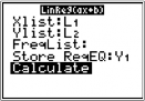
Fill in each argument in the stat wizard displayed.
Press [2nd] [L1] (for Xlist:), and [down key] [2nd] [L2] (for Ylist:), Press [down key] [down key] (to Store ReqEQ:)and then press
[ALPHA] [F4] [ENTER] to paste Y1. Press [down key] (to select Calculate).
Press [ENTER] to execute LinReg(ax+b). The linear regression for the data in L1 and L2 is calculated. Values for a and b are displayed in a temporary result screen. The linear regression equation is stored in Y1. Residuals are calculated and stored automatically in the list name RESID, which becomes an item on the LIST NAMES menu.
Note:
You can control the number of decimal places displayed by changing the decimal mode setting.
The statistics reported are not stored in the history on the home screen.
Press [VARS] 5 [right key] [right key] [right key]
to access the statistical variables.
Press [CLEAR] to return to the home screen.
The stat wizard pastes the populated command in the home screen history for repeated use, if needed (press [CLEAR] [up key] [up key] to view the home screen history as show in the screen).
Press [GRAPH]. The regression line and the scatter plot are displayed.
The regression line appears to fit the central portion of the scatter plot well. However, a residual plot may provide more information about this fit.
Press [STAT] 1 to select 1:Edit. The stat list editor is displayed.
Press [right key] and [up key] to move the cursor onto L3.
Press [2nd] [INS]. An unnamed column is displayed in column 3; L3, L4, L5, and L6 shift right one column. The Name= prompt is displayed in the entry line, and alpha-lock is on.
Press [2nd] [LIST] to display the LIST NAMES
menu.
If necessary, press [down key] to move the cursor onto the list name RESID.
Press [ENTER] to select RESID and paste it to the stat list editor’s Name= prompt.
Press [ENTER]. RESID is stored in column 3 of the stat list editor.
Press [down key] repeatedly to examine the residuals.
Notice that the first three residuals are negative. They correspond to the shortest pendulum string lengths in L1. The next five residuals are positive, and three of the last four are negative. The latter correspond to the longer string lengths in L1. Plotting the residuals will show this pattern more clearly.
Press [2nd] [STAT PLOT] 2 to select 2:Plot2 from the STAT PLOTS menu. The stat plot editor is displayed for plot 2.
Press [ENTER] to select On, which turns on plot 2.
Press [down key] [ENTER] to select scatter plot. Press [down key] [2nd] [L1] to specify Xlist:L1 for plot 2. Press [down key] [R] [E] [S] [I] [D]
(alpha-lock is on) to specify Ylist:RESID for plot 2. Press [down key] [ENTER] to select white square as the mark for each data point on the scatter plot.
Press [Y=] to display the Y= editor.
Press [left key] to move the cursor onto the = sign, and then press [ENTER] to deselect Y1. Press [up key] [ENTER] to turn off plot 1.
Press [ZOOM] 9 to select 9:ZoomStat from the ZOOM menu. The window variables are adjusted automatically, and plot 2 is displayed. This is a scatter plot of the residuals.
Notice the pattern of the residuals: a group of negative residuals, then a group of positive residuals, and then another group of negative residuals.
The residual pattern indicates a curvature associated with this data set for which the linear model did not account. The residual plot emphasizes a downward curvature, so a model that curves down with the data would be more accurate. Perhaps a function such as square root would fit. Try a power regression to fit a function of the form y = a * x to the b.
Press [Y=] to display the Y= editor.
Press [CLEAR] to clear the linear regression equation from Y1. Press [up key] [ENTER] to turn on plot 1. Press [right key] [ENTER] to turn off plot 2.

Press [ZOOM] 9 to select 9:ZoomStat from the ZOOM menu. The window variables are adjusted automatically, and the original scatter plot of time- versus-length data (plot 1) is displayed.
Press [STAT] [right key] [ALPHA] [A] to select A:PwrReg from the STAT CALC menu. PwrReg is pasted to the home screen.
Press [2nd] [L1] [down key] [2nd] [L2] [down
key] [down key] [ALPHA] [F4] [ENTER] [down key]
to highlight Calculate.
Note: You can also use the VARS Y-VARS FUNCTION menu, [VARS] [right key] 1 to select Y1.
Press [ENTER] to calculate the power regression.
Values for a and b are displayed on the home screen. The power regression equation is stored in Y1. Residuals are calculated and stored automatically in the list name RESID.
Press [GRAPH]. The regression line and the scatter plot are displayed.
The new function y =.192x to the 522 appears to fit the data well. To get more information, examine a residual plot.
Press [Y=] to display the Y= editor.
Press [left key][ENTER] to deselect Y1. Press [up key] [ENTER] to turn off plot 1. Press
[right key] [ENTER] to turn on plot 2.
Note: Step 19 defined plot 2 to plot residuals (RESID) versus string length (L1).
Press [ZOOM] 9 to select 9:ZoomStat from the ZOOM menu. The window variables are adjusted automatically, and plot 2 is displayed. This is a scatter plot of the residuals.
The new residual plot shows that the residuals are random in sign, with the residuals increasing in magnitude as the string length increases.
To see the magnitudes of the residuals, continue with these steps.
Press [TRACE].
Press [right key] and [left key] to trace the data. Observe the values for Y at each point.
With this model, the largest positive residual is about 0.041 and the smallest negative residual is about -0.027. All other residuals are less than 0.02 in magnitude.
Now that you have a good model for the relationship between length and period, you can use the model to predict the period for a given string length. To predict the periods for a pendulum with string lengths of 20 cm and 50 cm, continue with these steps.
Press [VARS] [right key] 1 to display the VARS Y-VARS FUNCTION secondary menu, and then press 1 to select 1:Y1. Y1 is pasted to the home screen.
Note: You can also use the YVARS ([ALPHA] [F4]) shortcut menu to select Y1.
Press [(]20 [)]to enter a string length of 20 cm.
Press [ENTER] to calculate the predicted time of about 0.92 seconds.
Based on the residual analysis, we would expect the prediction of about 0.92 seconds to be within about 0.02 seconds of the actual value.
Press [2nd] [ENTRY] to recall the Last Entry.
Press [left key] [left key] [left key] 5 to change the string length to 50 cm.
Press [ENTER] to calculate the predicted time of about 1.48 seconds.
Since a string length of 50 cm exceeds the lengths in the data set, and since residuals appear to be increasing as string length increases, we would expect more error with this estimate.
Note: You also can make predictions using the table with the TABLE SETUP settings Indpnt:Ask and Depend:Auto (Chapter 7).
Using Lists to Store Data
Data for statistical analyses is stored in lists, which you can create and edit using the stat list editor. The TI-84 Plus has six list variables in memory, L1 through L6, to which you can store data for statistical calculations. Also, you can store data to list names that you create (Chapter 11).
Setting Up a Statistical Analysis
To set up a statistical analysis, follow these steps. Read the chapter for details.
Enter the statistical data into one or more lists.
Plot the data.
Calculate the statistical variables or fit a model to the data.
Graph the regression equation for the plotted data.
Graph the residuals list for the given regression model.
Displaying the Stat List Editor
The stat list editor is a table where you can store, edit, and view up to 20 lists that are in memory. Also, you can create list names from the stat list editor.
To display the stat list editor, press [STAT], and then select 1:Edit from the STAT EDIT menu.
The top line displays list names. L1 through L6 are stored in columns 1 through 6 after a memory reset. The number of the current column is displayed in the top-right corner.
The bottom line is the entry line. All data entry occurs on this line. The characteristics of this line change according to the current context.
The center area displays up to seven elements of up to three lists; it abbreviates values when necessary. The entry line displays the full value of the current element.
Entering a List Name in the Stat List Editor
To enter a list name in the stat list editor, follow these steps.
Display the Name= prompt in the entry line in either of two ways.
Move the cursor onto the list name in the column where you want to insert a list, and then press [2nd] [INS]. An unnamed column is displayed and the remaining lists shift right one column.
Press [up key] until the cursor is on the top line, and then press [right key] until you reach the unnamed column.
Note: If list names are stored to all 20 columns, you must remove a list name to make room for an unnamed column.
The Name= prompt is displayed and alpha-lock is on.
Enter a valid list name in any of four ways.
Select a name from the LIST NAMES menu (Chapter 11).
Enter L1, L2, L3, L4, L5, or L6 from the keyboard.
Enter an existing user-created list name directly from the keyboard.
Enter a new user-created list name.
![]()
Press [ENTER] or [down key] to store the list name and its elements, if any, in the current column of the stat list editor.
To begin entering, scrolling, or editing list elements, press [down key]. The rectangular cursor is displayed.
Note: If the list name you entered in step 2 already was stored in another stat list editor column, then the list and its elements, if any, move to the current column from the previous column. Remaining list names shift accordingly.
Creating a Name in the Stat List Editor
To create a name in the stat list editor, follow these steps.
Display the Name= prompt.
Press [letter from A to Z or theta] to enter the first letter of the name. The first character cannot be a number.
Enter zero to four letters, theta, or numbers to complete the new user-created list name. List names can be one to five characters long.
Press [ENTER] or [down key] to store the list name in the current column of the stat list editor.
The list name becomes an item on the LIST NAMES menu (Chapter 11).
Removing a List from the Stat List Editor
To remove a list from the stat list editor, move the cursor onto the list name and then press [DEL]. The list is not deleted from memory; it is only removed from the stat list editor.
Notes:
To delete a list name from memory, use the MEMORY MANAGEMENT/DELETE secondary menu (Chapter 18).
If you archive a list, it will be removed from the stat list editor.
Removing All Lists and Restoring L1 through L6
You can remove all user-created lists from the stat list editor and restore list names L1 through L6
to columns 1 through 6 in either of two ways.
Use SetUpEditor with no arguments.
Reset all memory (Chapter 18).
Clearing All Elements from a List
You can clear all elements from a list in any of five ways.
Use ClrList to clear specified lists.
In the stat list editor, press [up key] to move the cursor onto a list name, and then press
[CLEAR] [ENTER].
In the stat list editor, move the cursor onto each element, and then press [DEL]one by one.
On the home screen or in the program editor, enter 0 right arrow dim(listname) to set the dimension of listname to 0 (Chapter 11).
Use ClrAllLists to clear all lists in memory (Chapter 18).
Editing a List Element
To edit a list element, follow these steps.
Move the cursor onto the element you want to edit.
Press [ENTER] to move the cursor to the entry line.
Note: If you want to replace the current value, you can enter a new value without first pressing
[ENTER]. When you enter the first character, the current value is cleared automatically.
Edit the element in the entry line.
Press one or more keys to enter the new value. When you enter the first character, the current value is cleared automatically.
You can use the shortcut menus to enter values. When you use n/d to enter a fraction, it is not displayed as a stacked fraction in the list. Instead, the fraction has a thick bar separating the numerator and denominator.
Thick-bar fraction on the list editor entry line:
![]() Thin-bar fraction on the home screen (regular
division):
Thin-bar fraction on the home screen (regular
division): ![]()
![]()
Note: Order of operations
applies to fractions. For example, evaluates to
![]() because the order of operations dictates that
division is performed before addition. To
because the order of operations dictates that
division is performed before addition. To
![]()
evaluate ![]() , enter with parentheses around the
numerator.
, enter with parentheses around the
numerator.
Press [right key] to move the cursor to the character before which you want to insert, press
[2nd] [INS], and then enter one or more characters.
Press [right key] to move the cursor to a character you want to delete, and then press [DEL]
to delete the character.
To cancel any editing and restore the original element at the rectangular cursor, press
[CLEAR] [ENTER].
Note: You can enter expressions and variables for elements.
Press [ENTER], [up key], or [down key] to update the list. If you entered an expression, it is evaluated. If you entered only a variable, the stored value is displayed as a list element.
When you edit a list element in the stat list editor, the list is updated in memory immediately.
Attaching a Formula to a List Name in Stat List Editor
You can attach a formula to a list name in the stat list editor, and then display and edit the calculated list elements. When executed, the attached formula must resolve to a list. Chapter 11 describes in detail the concept of attaching formulas to list names.
To attach a formula to a list name that is stored in the stat list editor, follow these steps.
Press [STAT] [ENTER] to display the stat list editor.
Press [up key] to move the cursor to the top line.
Press [left key] or [right key], if necessary, to move the cursor onto the list name to which you want to attach the formula.
Note: If a formula in quotation marks is displayed on the entry line, then a formula is already attached to the list name. To edit the formula, press [ENTER], and then edit the formula.
Press [ALPHA] ["], enter the formula, and press [ALPHA]["].
Note: If you do not use quotation marks, the TI-84 Plus calculates and displays the same initial list of answers, but does not attach the formula for future calculations.
Note: Any user-created list name referenced in a formula must be preceded by an L symbol (Chapter 11).
Press [ENTER]. The TI-84 Plus calculates each list element and stores it to the list name to which the formula is attached. A lock symbol is displayed in the stat list editor, next to the list name to which the formula is attached.
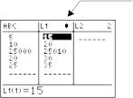
lock symbol
Using the Stat List Editor When Formula-Generated Lists Are Displayed
When you edit an element of a list referenced in an attached formula, the TI-84 Plus updates the corresponding element in the list to which the formula is attached (Chapter 11).
When a list with a formula attached is displayed in the stat list editor and you edit or enter elements of another displayed list, then the TI-84 Plus takes slightly longer to accept each edit or entry than when no lists with formulas attached are in view.
Note: To speed editing time, scroll horizontally until no lists with formulas are displayed, or rearrange the stat list editor so that no lists with formulas are displayed.
Handling Errors Resulting from Attached Formulas
On the home screen, you can attach to a list a formula that references another list with dimension 0 (Chapter 11). However, you cannot display the formula-generated list in the stat list editor or on the home screen until you enter at least one element to the list that the formula references.
All elements of a list referenced by an attached formula must be valid for the attached formula. For example, if Real number mode is set and the attached formula is log(L1), then each element of L1 must be greater than 0, since the logarithm of a negative number returns a complex result.
When you use the shortcut menus, all values must be valid for use in the templates. For example, if you use the n/d template, both the numerator and denominator must be integers.
Notes:
If an error menu is returned when you attempt to display a formula-generated list in the stat list editor, you can select 2:Goto, write down the formula that is attached to the list, and then press [CLEAR] [ENTER] to detach (clear) the formula. You then can use the stat list editor to find the
source of the error. After making the appropriate changes, you can reattach the formula to a list.
If you do not want to clear the formula, you can select 1:Quit, display the referenced list on the home screen, and find and edit the source of the error. To edit an element of a list on the home screen, store the new value to listname(element#) (Chapter 11).
Detaching a Formula from a List Name
You can detach (clear) a formula from a list name in several ways. For example:
In the stat list editor, move the cursor onto the name of the list to which a formula is attached.
Press [ENTER] [CLEAR] [ENTER]. All list elements remain, but the formula is detached and the lock symbol disappears.
In the stat list editor, move the cursor onto an element of the list to which a formula is attached.
Press [ENTER], edit the element, and then press [ENTER]. The element changes, the formula is detached, and the lock symbol disappears. All other list elements remain.
Use ClrList. All elements of one or more specified lists are cleared, each formula is detached, and each lock symbol disappears. All list names remain.
Use ClrAllLists (Chapter 18). All elements of all lists in memory are cleared, all formulas are detached from all list names, and all lock symbols disappear. All list names remain.
Editing an Element of a Formula-Generated List
As described above, one way to detach a formula from a list name is to edit an element of the list to which the formula is attached. The TI-84 Plus protects against inadvertently detaching the formula from the list name by editing an element of the formula-generated list.
Because of the protection feature, you must press [ENTER] before you can edit an element of a formula-generated list.
The protection feature does not allow you to delete an element of a list to which a formula is attached. To delete an element of a list to which a formula is attached, you must first detach the formula in any of the ways described above.
Stat List Editor Contexts
The stat list editor has four contexts.
View-elements context
View-names context
Edit-elements context
Enter-name context
The stat list editor is first displayed in view-elements context. To switch through the four contexts, select 1:Edit from the STAT EDIT menu and follow these steps.
Press [up key] to move the cursor onto a list name and switch to view-names context. Press [right key] and [left key] to view list names stored in other stat list editor columns.

Press [ENTER] to switch to edit-elements context.
You may edit any element in a list. All elements of the current list are displayed in braces ( { } ) in the entry line. Press [right key] and [left key] to view more list elements.
Press [ENTER] again to switch to view-elements context. Press [right key], [left key], [down key], and [up key] to view other list elements. The current element’s full value is displayed in the entry line.
Press [ENTER] again to switch back to edit- elements context. You may edit the current element in the entry line.
Press [up key] until the cursor is on a list name, then press [2nd] [INS] to switch to enter-name context.
Press [CLEAR] to switch to view-names context.
Press [down key] to switch back to view-elements context.
View-Elements Context
In view-elements context, the entry line displays the list name, the current element’s place in that list, and the full value of the current element, up to 12 characters at a time. An ellipsis (...) indicates that the element continues beyond 12 characters.

To page down the list six elements, press [ALPHA] [down key]. To page up six elements, press [ALPHA] [up key]. To delete a list element, press [DEL]. Remaining elements shift up one row. To insert a new element, press [2nd] [INS]. 0 is the default value for a new element.
Edit-Elements Context
In edit-elements context, the data displayed in the entry line depends on the previous context.
When you switch to edit-elements context from view-elements context, the full value of the current element is displayed. You can edit the value of this element, and then press [down key] and [up key] to edit other list elements.
![]()
When you switch to edit-elements context from view-names context, the full values of all elements in the list are displayed. An ellipsis indicates that list elements continue beyond the screen. You can press [right key] and [left key] to edit any element in the list.
![]()
Note: In edit-elements context, you can attach a formula to a list name only if you switched to it from view-names context.
View-Names Context
In view-names context, the entry line displays the list name and the list elements.

To remove a list from the stat list editor, press [DEL]. Remaining lists shift to the left one column. The list is not deleted from memory.
To insert a name in the current column, press [2nd] [INS]. Remaining columns shift to the right one column.
Enter-Name Context
In enter-name context, the Name= prompt is displayed in the entry line, and alpha-lock is on.
At the Name= prompt, you can create a new list name, paste a list name from L1 to L6 from the keyboard, or paste an existing list name from the LIST NAMES menu (Chapter 11). The L symbol is not required at the Name= prompt.
To leave enter-name context without entering a list name, press [CLEAR]. The stat list editor switches to view-names context.
STAT EDIT Menu
To display the STAT EDIT menu, press [STAT].
![]()
EDIT CALC TESTS
1: Edit... Displays the stat list editor.
2: SortA( Sorts a list in ascending order.
3: SortD( Sorts a list in descending order.
4: ClrList Deletes all elements of a list.
5: SetUpEditor Stores specified lists in the stat list editor.
![]()
SortA(, SortD(
SortA( (sort ascending) sorts list elements from low to high values. SortD( (sort descending) sorts list elements from high to low values. Complex lists are sorted based on magnitude (modulus). SortA( and SortD( each can sort in either of two ways.
With one listname, SortA( and SortD( sort the elements in listname and update the list in memory.
With two or more lists, SortA( and SortD( sort keylistname, and then sort each dependlist by placing its elements in the same order as the corresponding elements in keylistname. This lets you sort two-variable data on X and keep the data pairs together. All lists must have the same dimension.
The sorted lists are updated in memory.
SortA(listname) SortD(listname)
SortA(keylistname,dependlist1[,dependlist2,...,dependlist n])
SortD(keylistname,dependlist1[,dependlist2,...,dependlist n])
Note: SortA( and SortD( are the same as SortA( and SortD( on the LIST OPS menu.
ClrList
ClrList clears (deletes) from memory the elements of one or more listnames. ClrList also detaches any formula attached to a listname.
ClrList listname1,listname2,...,listname n
Note: To clear from memory all elements of all list names, use ClrAllLists (Chapter 18).
SetUpEditor
With SetUpEditor you can set up the stat list editor to display one or more listnames in the order that you specify. You can specify zero to 20 listnames.
Additionally, if you want to use listnames which happen to be archived, the SetUp Editor will automatically unarchive the listnames and place them in the stat list editor at the same time.
SetUpEditor [listname1,listname2,...,listname n]
SetUpEditor removes all list names from the stat list editor and then stores listnames in the stat list editor columns in the specified order, beginning in column 1.
![]()
MathPrintâ„¢
![]()
Classic 
If you enter a listname that is not stored in memory already, then listname is created and stored in memory; it becomes an item on the LIST NAMES menu.
Restoring L1 through L6 to the Stat List Editor
SetUpEditor with no listnames removes all list names from the stat list editor and restores list names
L1 through L6 in the stat list editor columns 1 through 6.
![]()
Regression Model Features
STAT CALC menu items 3 through C are regression models. The automatic residual list and automatic regression equation features apply to all regression models. Diagnostics display mode applies to some regression models.
Automatic Residual List
When you execute a regression model, the automatic residual list feature computes and stores the residuals to the list name RESID. RESID becomes an item on the LIST NAMES menu (Chapter 11).
![]()
The TI-84 Plus uses the formula below to compute RESID list elements. The next section describes the variable RegEQ.
RESID = Ylistname - RegEQ(Xlistname)
Automatic Regression Equation
Each regression model has an optional argument, regequ, for which you can specify a Y= variable such as Y1. Upon execution, the regression equation is stored automatically to the specified Y= variable and the Y= function is selected.
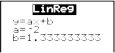
![]()
MathPrintâ„¢ MathPrintâ„¢ MathPrintâ„¢
Classic Classic
Regardless of whether you specify a Y= variable for regequ, the regression equation always is stored to the TI-84 Plus variable RegEQ, which is item 1 on the VARS Statistics EQ secondary menu.
![]()
Note: For the regression equation, you can use the fixed-decimal mode setting to control the number of digits stored after the decimal point (Chapter 1). However, limiting the number of digits to a small number could affect the accuracy of the fit.
Diagnostics Display Mode
When you execute some regression models, the TI-84 Plus computes and stores diagnostics values for r (correlation coefficient) and r square (coefficient of determination) or for R square (coefficient of determination). You can control whether these values are displayed by turning StatDiagnostics on or off on the mode screen.
r and r square are computed and stored for these regression models.
LinReg(ax+b) LinReg(a+bx)
LnReg ExpReg
PwrReg
R square is computed and stored for these regression models.
QuadReg CubicReg QuartReg
The r and r square that are computed for LnReg, ExpReg, and PwrReg are based on the linearly transformed data. For example, for ExpReg (y=ab^x), r and r square are computed on
ln y=ln a+x(ln b).
By default, these values are not displayed with the results of a regression model when you execute it. However, you can set the diagnostics display mode by executing the DiagnosticOn or DiagnosticOff instruction. Each instruction is in the CATALOG (Chapter 15).
To turn diagnostics on or off from the mode screen, select On or Off for StatDiagnostics. The default is Off.
To set DiagnosticOn or DiagnosticOff from the home screen, press [2nd] [CATALOG], and then select the instruction for the mode you want. The instruction is pasted to the home screen. Press [ENTER] to set the mode.
When DiagnosticOn is set, diagnostics are displayed with the results when you execute a regression model.
MathPrintâ„¢ 
Classic
When DiagnosticOff is set, diagnostics are not displayed with the results when you execute a regression model.
![]()
MathPrintâ„¢ 
Classic
STAT CALC Menu
To display the STAT CALC menu, press [STAT] [right key].
![]()
EDIT CALC TESTS
1: 1-Var Stats Calculates 1-variable statistics.
2: 2-Var Stats Calculates 2-variable statistics.
3: Med-Med Calculates a median-median line.
4: LinReg(ax+b) Fits a linear model to data.
5: QuadReg Fits a quadratic model to data.
6: CubicReg Fits a cubic model to data.
7: QuartReg Fits a quartic model to data.
8: LinReg(a+bx) Fits a linear model to data.
9: LnReg Fits a logarithmic model to data.
0: ExpReg Fits an exponential model to data.
A: PwrReg Fits a power model to data.
B: Logistic Fits a logistic model to data.
C: SinReg Fits a sinusoidal model to data.
D: Manual Linear Fit Fits a linear equation interactively to a scatter plot.
![]()
For each STAT CALC menu item, if neither Xlistname nor Ylistname is specified, then the default list names are L1 and L2. If you do not specify freqlist, then the default is 1 occurrence of each list element.
STAT WIZARDS in STAT CALC
When STAT WIZARDS is set to ON in MODE, a wizard will open by default. The wizard will prompt for required and optional arguments. In STAT CALC, select Calculate to paste the populated com- mand to home screen and display the results to a temporary view.
Note: After a calculation, statistical variables are available in the VARS menu.
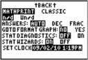
The following screens demonstrate the STAT WIZARDS flow for a STAT CALC menu command.
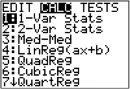
Press press [STAT] [right key] to select the STAT CALC menu. Select 1 [ENTER] to select the 1 -Var Stats menu.
Note: In this example, data has been entered in L1.
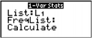
The 1 -Var Stats wizard opens. Enter the values in the wizard. Scroll down to Calculate and press [ENTER].
Note: FreqList is an optional argument.
The STAT CALC results are
displayed. 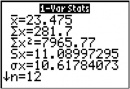
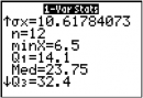
Press [down key] to scroll down through the data.
Note: This is a temporary view. Press [VARS] 5 to view the statistic variables after clearing the temporary result screen.
Press [CLEAR] to clear the data from the screen.
![]()
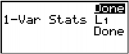
Press [up key] to view the populated command pasted.
If the STAT WIZARD mode option if OFF, for each STAT CALC menu item, if neither Xlistname nor Ylistname is specified, then the default list names are L1 and L2. If you do not specify freqlist, then the default is 1 occurrence of each list element.
Frequency of Occurrence for Data Points
For most STAT CALC menu items, you can specify a list of data occurrences, or frequencies (freqlist).
Each element in freqlist indicates how many times the corresponding data point or data pair occurs in the data set you are analyzing.
For example, if L1={15,12,9,14} and LFREQ={1,4,1,3}, then the TI-84 Plus interprets the instruction 1-Var Stats L1, LFREQ to mean that 15 occurs once, 12 occurs four times, 9 occurs once, and 14 occurs three times.
Each element in freqlist must be > (greater than or equal to) 0, and at least one element must be > (greater than) 0.
Noninteger freqlist elements are valid. This is useful when entering frequencies expressed as percentages or parts that add up to 1. However, if freqlist contains noninteger frequencies, Sx and Sy are undefined; values are not displayed for Sx and Sy in the statistical results.
1-Var Stats
1-Var Stats (one-variable statistics) analyzes data with one measured variable. Each element in freqlist is the frequency of occurrence for each corresponding data point in Xlistname. freqlist elements must be real numbers > (greater than) 0.
1-Var Stats [Xlistname,freqlist]
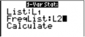
![]()
2-Var Stats
2-Var Stats (two-variable statistics) analyzes paired data. Xlistname is the independent variable. Ylistname is the dependent variable. Each element in freqlist is the frequency of occurrence for each data pair (Xlistname,Ylistname).
2-Var Stats [Xlistname,Ylistname,freqlist]
Med-Med (ax+b)
Med-Med (median-median) fits the model equation y = ax+b to the data using the median-median line (resistant line) technique, calculating the summary points x1, y1, x2, y2, x3, and y3. Med-Med displays values for a (slope) and b (y-intercept).
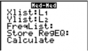
Med-Med [Xlistname,Ylistname,freqlist,regequ]
![]()
LinReg (ax+b)
LinReg(ax+b) (linear regression) fits the model equation y=ax+b to the data using a least-squares fit. It displays values for a (slope) and b (y-intercept); when DiagnosticOn is set, it also displays values for r square and r.
LinReg(ax+b) [Xlistname,Ylistname,freqlist,regequ]
QuadReg (ax square +bx+c)
QuadReg (quadratic regression) fits the second-degree polynomial y=ax square + bx + c to the data. It displays values for a, b, and c; when DiagnosticOn is set, it also displays a value for
R square. For three data points, the equation is a polynomial fit; for four or more, it is a polynomial regression. At least three data points are required.
QuadReg [Xlistname,Ylistname,freqlist,regequ]
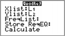
CubicReg—(ax cube+bx square +cx+d)
CubicReg (cubic regression) fits the third-degree polynomial y=ax cube+bx square +cx+d to the data. It displays values for a, b, c, and d; when DiagnosticOn is set, it also displays a value for
R square. For four points, the equation is a polynomial fit; for five or more, it is a polynomial regression. At least four points are required.
CubicReg [Xlistname,Ylistname,freqlist,regequ]
QuartReg—(ax to the 4+ bx cube + cx square + dx+e)
QuartReg (quartic regression) fits the fourth-degree polynomial y=ax to the 4+bx cube +cxsquare
+dx+e to the data. It displays values for a, b, c, d, and e; when DiagnosticOn is set, it also displays a value for R square. For five points, the equation is a polynomial fit; for six or more, it is a polynomial regression. At least five points are required.
QuartReg [Xlistname,Ylistname,freqlist,regequ]
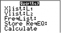
LinReg—(a+bx)
LinReg(a+bx) (linear regression) fits the model equation y=a+bx to the data using a least-squares fit. It displays values for a (y-intercept) and b (slope); when DiagnosticOn is set, it also displays values for r square and r.
LinReg(a+bx) [Xlistname,Ylistname,freqlist,regequ]
LnReg—(a+b ln(x))
LnReg (logarithmic regression) fits the model equation y=a+b ln(x) to the data using a least- squares fit and transformed values ln(x) and y. It displays values for a and b; when DiagnosticOn is set, it also displays values for r square and r.
LnReg [Xlistname,Ylistname,freqlist,regequ]
ExpReg—(ab to the x)
ExpReg (exponential regression) fits the model equation y=ab to the x to the data using a least- squares fit and transformed values x and ln(y). It displays values for a and b; when DiagnosticOn is set, it also displays values for r square and r.
ExpReg [Xlistname,Ylistname,freqlist,regequ]
PwrReg—(ax to the b)
PwrReg (power regression) fits the model equation y=ax to the b to the data using a least-squares fit and transformed values ln(x) and ln(y). It displays values for a and b; when DiagnosticOn is set, it also displays values for r square and r.
PwrReg [Xlistname,Ylistname,freqlist,regequ]
Logistic—c /(1+a*e to the -bx)
Logistic fits the model equation y=c/(1+a*e to the -bx) to the data using an iterative least-squares fit. It displays values for a, b, and c.
Logistic [Xlistname,Ylistname,freqlist,regequ]
SinReg—a sin(bx+c)+d
SinReg (sinusoidal regression) fits the model equation y=a sin(bx+c)+d to the data using an iterative least-squares fit. It displays values for a, b, c, and d. At least four data points are required. At least two data points per cycle are required in order to avoid aliased frequency estimates.
SinReg [iterations,Xlistname,Ylistname,period,regequ]
iterations is the maximum number of times the algorithm will iterate to find a solution. The value for iterations can be an integer > (greater than or equal to) 1 and < (less than or equal to)16; if not specified, the default is 3. The algorithm may find a solution before iterations is reached. Typically, larger values for iterations result in longer execution times and better accuracy for SinReg, and vice versa.
A period guess is optional. If you do not specify period, the difference between time values in Xlistname must be equal and the time values must be ordered in ascending sequential order. If you specify period, the algorithm may find a solution more quickly, or it may find a solution when it would not have found one if you had omitted a value for period. If you specify period, the differences between time values in Xlistname can be unequal.
Note: The output of SinReg is always in radians, regardless of the Radian/Degree mode setting.
SinReg Example: Daylight Hours in Alaska for One Year
Compute the regression model for the number of hours of daylight in Alaska during one year.
![]()
![]()
MathPrintâ„¢ 
Classic
![]()
![]()
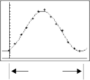
1 period
With noisy data, you will achieve better convergence results when you specify an accurate estimate for period. You can obtain a period guess in either of two ways.
Plot the data and trace to determine the x-distance between the beginning and end of one complete period, or cycle. The illustration above and to the right graphically depicts a complete period, or cycle.
Plot the data and trace to determine the x-distance between the beginning and end of N complete periods, or cycles. Then divide the total distance by N.
After your first attempt to use SinReg and the default value for iterations to fit the data, you may find the fit to be approximately correct, but not optimal. For an optimal fit, execute
SinReg 16,Xlistname,Ylistname,2pi/b where b is the value obtained from the previous SinReg
execution.
Manual Linear Fit
Manual Linear Fit allows you to visually fit a linear function to a scatter plot. Manual Linear Fit is an option in the [STAT] [CALC] menu.
After entering List data and viewing the StatPlot, select the Manual-Fit function.
Press [STAT] to display the Stat menu. Press [right key] to select CALC. Press [down key] several times to scroll down to select D:Manual-Fit. Press [ENTER]. This displays a free-floating cursor at the center of the display screen.
Press the cursor navigation keys ([up key] [down key] [left key] [right key] to move the cursor to the desired location. Press [ENTER] to select the first point.
Press the cursor navigation keys ([up key] [down key] [left key] [right key] to move the cursor to the second location. Press [ENTER]. This displays a line containing the two points selected.
The linear function is displayed. The Manual-Fit Line equation displays in the form of Y=mX+b. The current value of the first parameter (m) is highlighted in the symbolic expression.
Modify parameter values
Press the cursor navigation keys ( [left key][right key] ) to move from the first parameter (m) or (b) the second parameter. You can press [ENTER] and type a new parameter value. Press [ENTER] to display the new parameter value. When you edit the value of the selected parameter, the edit can include insert, delete, type over, or mathematical expression.
The screen dynamically displays the revised parameter value. Press [ENTER] to complete the modification of the selected parameter, save the value, and refresh the displayed graph. The system displays the revised parameter value in the symbolic expression Y=mX+B, and refreshes the graph with the updated Manual-Fit Line.
Select [2nd] [QUIT] to finish the Manual Fit function. The calculator stores the current mX+b expression into Y1 and makes that function active for graphing. You can also select Manual-Fit while on the Home screen. You can then enter a different Y-Var such as Y4 and then press [ENTER]. This takes you to the Graph screen and then pastes the Manual-Fit equation in the specified Y-Var. In this example, Y4.
The statistical variables are calculated and stored as indicated below. To access these variables for use in expressions, press [VARS], and select 5:Statistics. Then select the VARS menu shown in the column below under VARS menu. If you edit a list or change the type of analysis, all statistical variables are cleared.
|
Variables |
1-Var Stats |
2-Var Stats |
Other |
VARS menu |
|
mean of x values |
x (x bar) |
x (x bar) |
XY |
|
|
sum of x values |
Sigma x |
Sigma x |
Sigma |
|
|
sum of x square values |
Sigma x square |
Sigma x square |
Sigma |
|
|
sample standard deviation of x |
Sx |
Sx |
XY |
|
|
population standard deviation of x |
small sigma x |
small sigma x |
XY |
|
|
number of data points |
n |
n |
XY |
|
|
mean of y values |
y ( y bar) |
XY |
||
|
sum of y values |
Sigma y |
Sigma |
||
|
sum of y square values |
Sigma y square |
Sigma |
||
|
sample standard deviation of y |
Sy |
XY |
||
|
population standard deviation of y |
small sigma y |
XY |
||
|
sum of x * y |
Sigma xy |
Sigma |
||
|
minimum of x values |
minX |
minX |
XY |
|
|
maximum of x values |
maxX |
maxX |
XY |
|
|
minimum of y values |
minY |
XY |
||
|
maximum of y values |
maxY |
XY |
||
|
1st quartile |
Q1 |
PTS |
||
|
median |
Med |
PTS |
||
|
3rd quartile |
Q3 |
PTS |
|
Variables |
1-Var Stats |
2-Var Stats |
Other |
VARS menu |
|
regression/fit coefficients |
a, b |
EQ |
||
|
polynomial, Logistic, and SinReg coefficients |
a, b, c, d, e |
EQ |
||
|
correlation coefficient |
r |
EQ |
||
|
coefficient of determination |
r square, R square |
EQ |
||
|
regression equation |
RegEQ |
EQ |
||
|
summary points (Med-Med only) |
x1, y1, x2, y2, x3, y3 |
PTS |
Q1 and Q3
The first quartile (Q1) is the median of points between minX and Med (median). The third quartile (Q3) is the median of points between Med and maxX.
Entering Stat Data
You can enter statistical data, calculate statistical results, and fit models to data from a program. You can enter statistical data into lists directly within the program (Chapter 11).
![]()
Statistical Calculations
To perform a statistical calculation from a program, follow these steps.
On a blank line in the program editor, select the type of calculation from the STAT CALC menu.
Enter the names of the lists to use in the calculation. Separate the list names with a comma.
Enter a comma and then the name of a Y= variable, if you want to store the regression equation to a Y= variable.
Steps for Plotting Statistical Data in Lists
You can plot statistical data that is stored in lists. The six types of plots available are scatter plot, xyLine, histogram, modified box plot, regular box plot, and normal probability plot. You can define up to three plots.
To plot statistical data in lists, follow these steps.
Store the stat data in one or more lists.
Select or deselect Y= functions as appropriate.
Define the stat plot.
Turn on the plots you want to display.
Define the viewing window.
Display and explore the graph.
Scatter
Scatter plots plot the data points from Xlist and Ylist as coordinate pairs, showing each point as a box, cross ( + ), or dot. Xlist and Ylist must be the same length. You can use the same list for Xlist and Ylist.

xyLine
xyLine is a scatter plot in which the data points are plotted and connected in order of appearance in Xlist and Ylist. You may want to use SortA( or SortD( to sort the lists before you plot them.
Histogram
Histogram plots one-variable data. The Xscl window variable value determines the width of each bar, beginning at Xmin. ZoomStat adjusts Xmin, Xmax, Ymin, and Ymax to include all values, and also adjusts Xscl. The inequality (Xmax - Xmin) / Xscl < (less than or equal to) 47 must be true. A value that occurs on the edge of a bar is counted in the bar to the right.
ModBoxplot
ModBoxplot (modified box plot) plots one-variable data, like the regular box plot, except points that are 1.5 * Interquartile Range beyond the quartiles. (The Interquartile Range is defined as the difference between the third quartile Q3 and the first quartile Q1.) These points are plotted individually beyond the whisker, using the Mark (white square or + or black dot) you select. You can trace these points, which are called outliers.
The prompt for outlier points is x=, except when the outlier is the maximum point (maxX) or the minimum point (minX). When outliers exist, the end of each whisker will display x=. When no outliers exist, minX and maxX are the prompts for the end of each whisker. Q1, Med (median), and Q3 define the box.
Box plots are plotted with respect to Xmin and Xmax, but ignore Ymin and Ymax. When two box plots are plotted, the first one plots at the top of the screen and the second plots in the middle. When three are plotted, the first one plots at the top, the second in the middle, and the third at the bottom.
Boxplot
Boxplot (regular box plot) plots one-variable data. The whiskers on the plot extend from the minimum data point in the set (minX) to the first quartile (Q1) and from the third quartile (Q3) to the maximum point (maxX). The box is defined by Q1, Med (median), and Q3.
Box plots are plotted with respect to Xmin and Xmax, but ignore Ymin and Ymax. When two box plots are plotted, the first one plots at the top of the screen and the second plots in the middle.
When three are plotted, the first one plots at the top, the second in the middle, and the third at the bottom.
NormProbPlot
NormProbPlot (normal probability plot) plots each observation X in Data List versus the corresponding quantile z of the standard normal distribution. If the plotted points lie close to a straight line, then the plot indicates that the data are normal.
Enter a valid list name in the Data List field. Select X or Y for the Data Axis setting.
If you select X, the TI-84 Plus plots the data on the x-axis and the z-values on the y-axis.
If you select Y, the TI-84 Plus plots the data on the y-axis and the z-values on the x-axis.
Defining the Plots
To define a plot, follow these steps.
Press [2nd] [STAT PLOT]. The STAT PLOTS menu is displayed with the current plot definitions.
Select the plot you want to use. The stat plot editor is displayed for the plot you selected.

Press [ENTER] to select On if you want to plot the statistical data immediately. The definition is stored whether you select On or Off.
Select the type of plot. Each type prompts for the options checked in this table.
![]()
Plot Type XList YList Mark Freq
![]()
Scatter checked checked checked
![]()
xyLine checked checked checked
![]()
Histogram checked checked
![]()
ModBoxplot checked checked checked
![]()
Boxplot checked checked
Data List
Data Axis
![]()
NormProbPlot checked checked checked
![]()
Enter list names or select options for the plot type.
Xlist (list name containing independent data)
Ylist (list name containing dependent data)
Mark (white square or + or black dot)
Freq (frequency list for Xlist elements; default is 1)
Data List (list name for NormProbPlot)
Data Axis (axis on which to plot Data List)
Displaying Other Stat Plot Editors
Each stat plot has a unique stat plot editor. The name of the current stat plot (Plot1, Plot2, or Plot3) is highlighted in the top line of the stat plot editor. To display the stat plot editor for a different plot, press [up key] and [right key] to move the cursor onto the name in the top line, and then press [ENTER]. The stat plot editor for the selected plot is displayed, and the selected name remains highlighted.

Turning On and Turning Off Stat Plots
PlotsOn and PlotsOff allow you to turn on or turn off stat plots from the home screen or a program. With no plot number, PlotsOn turns on all plots and PlotsOff turns off all plots. With one or more plot numbers (1, 2, and 3), PlotsOn turns on specified plots, and PlotsOff turns off specified plots.
PlotsOff [1,2,3]
PlotsOn [1,2,3]
Note: You also can turn on and turn off stat plots in the top line of the Y= editor (Chapter 3).
Defining the Viewing Window
Stat plots are displayed on the current graph. To define the viewing window, press [WINDOW] and enter values for the window variables. ZoomStat redefines the viewing window to display all statistical data points.
Tracing a Stat Plot
When you trace a scatter plot or xyLine, tracing begins at the first element in the lists.
When you trace a histogram, the cursor moves from the top center of one column to the top center of the next, starting at the first column.
When you trace a box plot, tracing begins at Med (the median). Press [left key] to trace to Q1 and
minX. Press [right key] to trace to Q3 and maxX.
When you press [up key] or [down key] to move to another plot or to another Y= function, tracing moves to the current or beginning point on that plot (not the nearest pixel).
The ExprOn/ExprOff format setting applies to stat plots (Chapter 3). When ExprOn is selected, the plot number and plotted data lists are displayed in the top-left corner.
Defining a Stat Plot in a Program
To display a stat plot from a program, define the plot, and then display the graph.
To define a stat plot from a program, begin on a blank line in the program editor and enter data into one or more lists; then, follow these steps.
Press [2nd] [STAT PLOT] to display the STAT PLOTS menu.
Select the plot to define, which pastes Plot1(, Plot2(, or Plot3( to the cursor location.
![]()
Press [2nd] [STAT PLOT] [right key] to display the STAT TYPE menu.
Select the type of plot, which pastes the name of the plot type to the cursor location.
![]()
Press [,]. Enter the list names, separated by commas.
Press [,] [2nd] [STAT PLOT] [left key] to display the STAT PLOT MARK menu. (This step is not necessary if you selected 3:Histogram or 5:Boxplot in step 4.)
![]()
Select the type of mark (white square or + or white dot) for each data point. The selected mark symbol is pasted to the cursor location.
Press [)][ENTER] to complete the command line.
Displaying a Stat Plot from a Program
To display a plot from a program, use the DispGraph instruction (Chapter 16) or any of the ZOOM instructions (Chapter 3).
Getting Started is a fast-paced introduction. Read the chapter for details.
Suppose you want to estimate the mean height of a population of women given the random sample below. Because heights among a biological population tend to be normally distributed, a t distribution confidence interval can be used when estimating the mean. The 10 height values below are the first 10 of 90 values, randomly generated from a normally distributed population with an assumed mean of 165.1 centimeters and a standard deviation of 6.35 centimeters (randNorm(165.1,6.35,90) with a seed of 789).
Height (in centimeters) of Each of 10 Women
169.43 168.33 159.55 169.97 159.79 181.42 171.17 162.04 167.15 159.53

Press [STAT] [ENTER] to display the stat list editor.
Press [up key] to move the cursor onto L1, and then press [2nd] [INS] to insert a new list. The Name= prompt is displayed on the bottom line. The reverse A cursor indicates that alpha-lock is on. The existing list name columns shift to the right.
Note: Your stat editor may not look like the one pictured here, depending on the lists you have already stored.
Enter [H] [G] [H] [T] at the Name= prompt, and then press [ENTER] to create the list to store the women’s height data.
Press [down key] to move the cursor into the first row of the list. HGHT(1)= is displayed on the bottom line. Press [ENTER].
Press 169 [.] 43 to enter the first height value. As you enter it, it is displayed on the bottom line.
Press [ENTER]. The value is displayed in the first row, and the rectangular cursor moves to the next row.
Enter the other nine height values the same way.
Press [STAT] [left key] to display the STAT TESTS menu, and then press [down key] until 8:TInterval is highlighted.
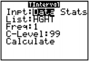
Press [ENTER] to select 8:TInterval. The inferential stat editor for TInterval is displayed. If Data is not selected for Inpt:, press [left key] [ENTER] to select Data.
Press [down key] [2nd] [LIST] and press [down key]
until HGHT is highlighted and then press [ENTER].
Press [down key] [down key] [.] 99 to enter a 99 percent confidence level at the C-Level: prompt.
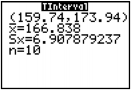
Press [down key] to move the cursor onto Calculate, and then press [ENTER]. The confidence interval is calculated, and the TInterval results are displayed on the home screen.
Interpreting the results
The first line, (159.74,173.94), shows that the 99 percent confidence interval for the population mean is between about 159.74 centimeters and 173.94 centimeters. This is about a 14.2 centimeters spread.
The .99 confidence level indicates that in a very large number of samples, we expect 99 percent of the intervals calculated to contain the population mean. The actual mean of the population sampled is 165.1 centimeters, which is in the calculated interval.
The second line gives the mean height of the sample mean of x used to compute this interval. The third line gives the sample standard deviation Sx. The bottom line gives the sample size n.
To obtain a more precise bound on the population mean (mu) of women’s heights, increase the sample size to 90. Use a sample mean of x of 163.8 and sample standard deviation Sx of 7.1 calculated from the larger random sample. This time, use the Stats (summary statistics) input option.
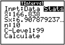
Press [STAT] [left key] 8 to display the inferential stat editor for TInterval.
Press [right key] [ENTER] to select Inpt:Stats. The editor changes so that you can enter summary statistics as input.
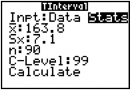
Press [down key] 163 [.] 8 [ENTER] to store 163.8 to mean of x.
Press 7 [.] 1 [ENTER] to store 7.1 to Sx. Press 90 [ENTER] to store 90 to n.
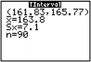
Press [down key] to move the cursor onto Calculate, and then press [ENTER] to calculate the new 99 percent confidence interval. The results are displayed on the home screen.
If the height distribution among a population of women is normally distributed with a mean (mu) of
165.1 centimeters and a standard deviation s of 6.35 centimeters, what height is exceeded by only 5 percent of the women (the 95th percentile)?
Press [CLEAR] to clear the home screen.
Press [2nd][DISTR] to display the DISTR
(distributions) menu.
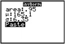
Press 3 to open the invNorm( wizard. Enter the information as follows:
Press [.] 95 [down key] 165 [.] 1 [down key] 6 [.] 35 [down key] (95 is the area, 165.1 is mu, and 6.35 is small sigma).
Press [ENTER] to paste the function and [ENTER]
again to calculate the result.
The result is displayed on the home screen; it shows that five percent of the women are taller than
175.5 centimeters.
Now graph and shade the top 5 percent of the population.
Press [WINDOW] and set the window variables to these values.
Xmin=145 Ymin=-.02 Xres=1 Xmax=185 Ymax=.08
Xscl=5 Yscl=0
Press [2nd] [DISTR] [right key] to display the
DISTR DRAW menu.
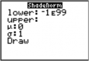
Press [ENTER] to open a wizard for the input of the ShadeNorm( parameters.
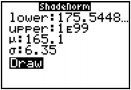
Enter 175 [.] 5448205 for the lower bound and press [down key]. Enter 1 [2nd] [EE] 99 for the upper bound and press [down key]. Enter the mean mu of 165 [.] 1 for the normal curve and press [down key]. Enter a standard deviation small sigma of 6 [.] 35.
Press [down key] to select Draw and then press
[ENTER] to plot and shade the normal curve.
Area is the area above the 95th percentile. low is the lower bound. up is the upper bound.
Displaying the Inferential Stat Editors
When you select a hypothesis test or confidence interval instruction from the home screen, the appropriate inferential statistics editor is displayed. The editors vary according to each test or interval’s input requirements. Below is the inferential stat editor for T-Test.
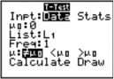
Note: When you select the ANOVA( instruction, it is pasted to the home screen. ANOVA( does not have an editor screen.
Using an Inferential Stat Editor
To use an inferential stat editor, follow these steps.
Select a hypothesis test or confidence interval from the STAT TESTS menu. The appropriate editor is displayed.
Select Data or Stats input, if the selection is available. The appropriate editor is displayed.
Enter real numbers, list names, or expressions for each argument in the editor.
Select the alternative hypothesis (not equal to, less than, or greater than) against which to test, if the selection is available.
Select No or Yes for the Pooled option, if the selection is available.
Select Calculate or Draw (when Draw is available) to execute the instruction.
When you select Calculate, the results are displayed on the home screen.
When you select Draw, the results are displayed in a graph.
This chapter describes the selections in the above steps for each hypothesis test and confidence interval instruction.
Select Data or Stats input
Enter values
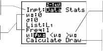
Select an alternative hypothesis
for arguments Select
Calculate or
Draw output
Selecting Data or Stats
Most inferential stat editors prompt you to select one of two types of input. (1-PropZInt and 2-PropZTest, 1-PropZInt and 2-PropZInt, chi square-Test, chi square GOF-Test, LinRegTInt, and LinRegTTest do not.)
Select Data to enter the data lists as input.
Select Stats to enter summary statistics, such as the mean of x, Sx, and n, as input. To select Data or Stats, move the cursor to either Data or Stats, and then press [ENTER]. Entering the Values for Arguments
Inferential stat editors require a value for every argument. If you do not know what a particular argument symbol represents, see the Inferential Statistics Input Descriptions tables.
When you enter values in any inferential stat editor, the TI-84 Plus stores them in memory so that you can run many tests or intervals without having to reenter every value.
Selecting an Alternative Hypothesis (not equal to, less than, or greater than)
Most of the inferential stat editors for the hypothesis tests prompt you to select one of three alternative hypotheses.
The first is a not equal to alternative hypothesis, such as mu not equal to mu0 for the Z-Test.
The second is a less than alternative hypothesis, such as mu1 less than mu2 for the
2-SampTTest.
The third is a greater than alternative hypothesis, such as p1 greater than p2 for the
2-PropZTest.
To select an alternative hypothesis, move the cursor to the appropriate alternative, and then press
[ENTER].
Selecting the Pooled Option
Pooled (2-SampTTest and 2-SampTInt only) specifies whether the variances are to be pooled for the calculation.
Select No if you do not want the variances pooled. Population variances can be unequal.
Select Yes if you want the variances pooled. Population variances are assumed to be equal. To select the Pooled option, move the cursor to Yes, and then press [ENTER].
Selecting Calculate or Draw for a Hypothesis Test
After you have entered all arguments in an inferential stat editor for a hypothesis test, you must select whether you want to see the calculated results on the home screen (Calculate) or on the graph screen (Draw).
Calculate calculates the test results and displays the outputs on the home screen.
Draw draws a graph of the test results and displays the test statistic and p-value with the graph. The window variables are adjusted automatically to fit the graph.
To select Calculate or Draw, move the cursor to either Calculate or Draw, and then press [ENTER]. The instruction is immediately executed.
Selecting Calculate for a Confidence Interval
After you have entered all arguments in an inferential stat editor for a confidence interval, select
Calculate to display the results. The Draw option is not available.
When you press [ENTER], Calculate calculates the confidence interval results and displays the outputs on the home screen.
Bypassing the Inferential Stat Editors
To paste a hypothesis test or confidence interval instruction to the home screen without displaying the corresponding inferential stat editor, select the instruction you want from the CATALOG menu. Appendix A describes the input syntax for each hypothesis test and confidence interval instruction.
![]()
Note: You can paste a hypothesis test or confidence interval instruction to a command line in a program. From within the program editor, select the instruction from either the CATALOG (Chapter 15) or the STAT TESTS menu.
STAT TESTS Menu
To display the STAT TESTS menu, press [STAT] [left key]. When you select an inferential statistics instruction, the appropriate inferential stat editor is displayed.
Most STAT TESTS instructions store some output variables to memory. For a list of these variables, see the Test and Interval Output Variables table.
![]()
EDIT CALC TESTS
1: Z-Test... Test for 1 mu, known small sigma
2: T-Test... Test for 1 mu, unknown small sigma
3: 2-SampZTest... Test comparing 2 mu’s, known small sigma’s 4: 2-SampTTest... Test comparing 2 mu’s, unknown small sigma’s 5: 1-PropZTest... Test for 1 proportion
6: 2-PropZTest... Test comparing 2 proportions
7: ZInterval... Confidence interval for 1 mu, known small sigma
8: TInterval... Confidence interval for 1 mu, unknown small sigma
9: 2-SampZInt... Confidence interval for difference of 2 mu’s, known small
sigma’s
0: 2-SampTInt... Confidence interval for difference of 2 mu’s, unknown small
sigma’s
A: 1-PropZInt... Confidence interval for 1 proportion
B: 2-PropZInt... Confidence interval for difference of 2 proportions
C: chi square-Test... Chi-square test for 2-way tables
D: chi square-GOF Test...
Chi-square Goodness of Fit test
E: 2-SampFTest... Test comparing 2 selections (small sigma’s)
F: LinRegTTest... t test for regression slope and rho
G: LinRegTInt... Confidence interval for linear regression slope coefficient b
H: ANOVA( One-way analysis of variance
![]()
Note: When a new test or interval is computed, all previous output variables are invalidated.
Inferential Stat Editors for the STAT TESTS Instructions
In this chapter, the description of each STAT TESTS instruction shows the unique inferential stat editor for that instruction with example arguments.
Descriptions of instructions that offer the Data/Stats input choice show both types of input screens.
Descriptions of instructions that do not offer the Data/Stats input choice show only one input screen.
The description then shows the unique output screen for that instruction with the example results.
Descriptions of instructions that offer the Calculate/Draw output choice show both types of screens: calculated and graphic results.
Descriptions of instructions that offer only the Calculate output choice show the calculated results on the home screen.
Z-Test
Z-Test (one-sample z test; item 1) performs a hypothesis test for a single unknown population mean mu when the population standard deviation small sigma is known. It tests the null hypothesis H subscript 0: mu=mu subscript 0 against one of the alternatives below.
H subscripta: mu not equal to mu subscript 0 (mu: not equal to mu0)
H subscripta: mu less than mu subscript 0 (mu: less than mu0)
H subscripta: mu greater than m subscript 0 (mu: greater than mu0) In the example:
L1={299.4, 297.7, 301, 298.9, 300.2, 297}
Data Stats
Input: 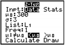
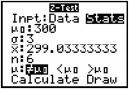
![]()
![]()
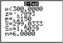
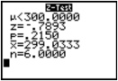
Calculated
results:
![]()
![]()
Drawn results:
Note: All STAT TESTS examples assume a fixed-decimal mode setting of 4 (Chapter 1). If you set the decimal mode to Float or a different fixed-decimal setting, your output may differ from the output in the examples.
T-Test
T-Test (one-sample t test; item 2) performs a hypothesis test for a single unknown population mean mu when the population standard deviation small sigma is unknown. It tests the null hypothesis H subscript 0: mu = mu subscript 0 against one of the alternatives below.
H subscript a: mu not equal to mu subscript 0 (mu: not equal to mu0)
H subscript a: mu less than mu subscript 0 (mu: less than mu0)
H subscript a: mu greater than mu subscript 0 (mu: greater than mu0) In the example:
TEST={91.9, 97.8, 111.4, 122.3, 105.4, 95}
Data Stats
Input: 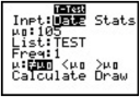
![]()
![]()
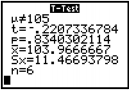
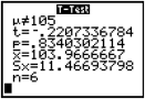
Calculated
results:
![]()
![]()

Drawn results:
2-SampZTest
2-SampZTest (two-sample z test; item 3) tests the equality of the means of two populations (mu subscript 1 and mu subscript 2) based on independent samples when both population standard deviations (small sigma subscript 1 and small sigma subscript 2) are known. The null hypothesis H subscript 0: mu subscript 1 =mu subscript 2 is tested against one of the alternatives below.
H subscript a: mu subscript 1 not equal to mu subscript 2 (mu1: not equal to mu2)
H subscript a: mu subscript 1 less than mu subscript 2 (mu1: less than mu2)
H subscript a: mu subscript 1 greater than subscript 2 (mu1: greater than mu2) In the example:
LISTA={154, 109, 137, 115, 140}
LISTB={108, 115, 126, 92, 146}
Data Stats
Input: 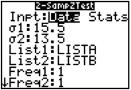
![]()
![]()
![]()
![]()
Calculated
results:
![]()
![]()
![]()
![]()

Drawn results:
2-SampTTest
2-SampTTest (two-sample t test; item 4) tests the equality of the means of two populations (mu subscript 1 and mu subscript 2) based on independent samples when neither population standard deviation (small sigma subscript 1 or small sigma subscript 2) is known. The null hypothesis H subscript 0: mu subscript 1=mu subscript 2 is tested against one of the alternatives below.
H subscript a: mu subscript 1 is not equal to mu subscript 2 (mu1: not equal to mu2)
H subscript a: mu subscript 1 less than mu subscript 2 (mu1: less than mu2)
H subscript a: mu subscript 1 greater than mu subscript 2 (mu1: greater than mu2) In the example:
SAMP1={12.207, 16.869, 25.05, 22.429, 8.456, 10.589}
SAMP2={11.074, 9.686, 12.064, 9.351, 8.182, 6.642}
Data Stats
Input: 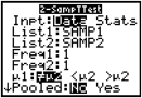
![]()
![]()
![]()
![]()
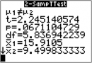
Calculated
results:

![]()
![]()

Drawn results:
1-PropZTest
PropZTest (one-proportion z test; item 5) computes a test for an unknown proportion of successes (prop). It takes as input the count of successes in the sample x and the count of observations in the sample n. 1-PropZTest tests the null hypothesis H subscript 0: prop=p subscript 0 against one of the alternatives below.
H subscript a: prop is not equal to p subscript 0 (prop: is not equal to p0)
H subscript a: prop is less than p subscript 0 (prop: is less than p0)
H subscript a: prop is greater than p subscript 0 (prop: is greater than p0)
Input: 
![]()
Calculated
results:
![]()
Drawn results:
2-PropZTest
PropZTest (two-proportion z test; item 6) computes a test to compare the proportion of successes (p subscript 1 and p subscript 2) from two populations. It takes as input the count of successes in each sample (x subscript 1 and x subscript 2) and the count of observations in each sample (n subscript 1 and n subscript 2). 2-PropZTest tests the null hypothesis H subscript 0: p subscript 1= p subscript 2 (using the pooled sample proportion) against one of the alternatives below.
H subscript a: p subscript 1 is not equal to p subscript 2 (p1: is not equal to p2)
H subscript a: p subscript 1 is less than p subscript 2 (p1: is less than p2)
H subscript a: p subscript 1 is greater than p subscript 2 (p1: is greater than p2)
Input: 
![]()
Calculated
results:
![]()
![]()
Drawn results:
ZInterval
ZInterval (one-sample z confidence interval; item 7) computes a confidence interval for an unknown population mean (mu) when the population standard deviation small sigma is known. The computed confidence interval depends on the user-specified confidence level.
In the example:
L1={299.4, 297.7, 301, 298.9, 300.2, 297}
Data Stats
Input: 
![]()
![]()
Calculated
results:
TInterval
TInterval (one-sample t confidence interval; item 8) computes a confidence interval for an unknown population mean (mu) when the population standard deviation small sigma is unknown. The computed confidence interval depends on the user-specified confidence level.
In the example:
L6={1.6, 1.7, 1.8, 1.9}
Data Stats
![]()
Input:
![]()
Data Stats
Calculated
results:
2-SampZInt
2-SampZInt (two-sample z confidence interval; item 9) computes a confidence interval for the difference between two population means (mu subscript 1 - mu subscript 2) when both population standard deviations (small sigma subscript 1 and small sigma subscript 2) are known. The computed confidence interval depends on the user-specified confidence level.
In the example:
LISTC={154, 109, 137, 115, 140}
LISTD={108, 115, 126, 92, 146}
Data Stats
Input: 
![]()
![]()
![]()
![]()
Calculated
results:
![]()
2-SampTInt
2-SampTInt (two-sample t confidence interval; item 0) computes a confidence interval for the difference between two population means (mu subscript 1 - mu subscript 2) when both population standard deviations (small sigma subscript 1 and small sigma subscript 2) are unknown. The computed confidence interval depends on the user-specified confidence level.
In the example:
SAMP1={12.207, 16.869, 25.05, 22.429, 8.456, 10.589}
SAMP2={11.074, 9.686, 12.064, 9.351, 8.182, 6.642}
Data Stats
Input: 
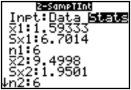
![]()
![]()
![]()
![]()
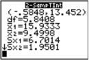
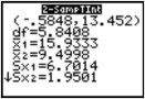
Calculated
![]()
results:
![]()
1-PropZInt
PropZInt (one-proportion z confidence interval; item A) computes a confidence interval for an unknown proportion of successes. It takes as input the count of successes in the sample x and the count of observations in the sample n. The computed confidence interval depends on the user- specified confidence level.
Input: 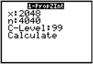
![]()
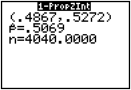
Calculated
results:
2-PropZInt
PropZInt (two-proportion z confidence interval; item B) computes a confidence interval for the difference between the proportion of successes in two populations (p subscript 1 - p subscript 2). It takes as input the count of successes in each sample (x subscript 1 and x subscript 2) and the count of observations in each sample (n subscript 1 and n subscript 2). The computed confidence interval depends on the user-specified confidence level.
Input: 
![]()
Calculated
results:
Chi square-Test
Chi square-Test (chi-square test; item C) computes a chi-square test for association on the two-way table of counts in the specified Observed matrix. The null hypothesis H subscript 0 for a two-way table is: no association exists between row variables and column variables. The alternative hypothesis is: the variables are related.
Before computing a Chi square-Test, enter the observed counts in a matrix. Enter that matrix variable name at the Observed: prompt in the Chi square-Test editor; default=[A]. At the Expected: prompt, enter the matrix variable name to which you want the computed expected counts to be stored; default=[B].
Matrix editor:
Input:
Note: Press [2nd] [MATRX] [right key] [right key] 1 to select 1:[A] from the MATRX EDIT menu.
Note: Press [2nd] [MATRX] [down key] [ENTER] to display matrix [B].
![]()
Calculated
results:
![]()
Drawn results:
Chi Square GOF-Test
Chi Square GOF-Test (Chi Square Goodness of Fit; item D) performs a test to confirm that sample data is from a population that conforms to a specified distribution. For example, Chi Square GOF can confirm that the sample data came from a normal distribution.
In the example:
list 1={16, 25, 22, 8, 10}
list 2={16.2, 21.6, 16.2, 14.4, 12.6}
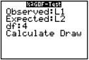
The Chi-square Goodness of Fit input screen:
![]()
Calculated
results:
![]()
Drawn results:
Note: Press [STAT] [right key] [right key] to select TESTS. Press [down key] several times to select D:XsquareGOF-Test... Press [ENTER]. To enter data for df (degree of freedom), press [down key] [down key] [down key]. Type 4.
2-SampFTest
2-SampFTest (two-sample F-test; item E) computes an F-test to compare two normal population standard deviations (small sigma subscript 1 and small sigma subscript 2). The population means and standard deviations are all unknown.
2-SampFTest, which uses the ratio of sample variances Sx1 square/Sx2square, tests the null hypothesis H subscript 0: s1=s2 against one of the alternatives below.
Ha: small sigma subscript 1 is not equal to small sigma subscript 2 (selection1 : not equal to
selection2)
Ha: small sigma subscript 1 is less than small sigma subscript 2 (selection1 : less than selection2)
Ha: small sigma subscript 1 is greater than small sigma subscript 2 (selection1 : greater than
selection2) In the example:
SAMP4={7,-4, 18, 17, -3, -5, 1, 10, 11, -2}
SAMP5={-1, 12, -1, -3, 3, -5, 5, 2, -11, -1, -3}
Data Stats
Input: 
![]()
![]()
Calculated
results:
![]()
![]()
![]()
![]()

Drawn results:
LinRegTTest
LinRegTTest (linear regression t test; item F) computes a linear regression on the given data and a t test on the value of slope Beta and the correlation coefficient rho for the equation y=a+Betax. It tests the null hypothesis H subscript 0: Beta =0 (equivalently, rho=0) against one of the alternatives below.
H subscript a: Beta is not equal to 0 and rho is not equal to 0 (Beta & rho: is not equal to 0)
H subscript a: Beta is less than 0 and rho is less than 0 (Beta & rho: is less than 0)
H subscript a: Beta is greater than 0 and rho is greater than 0 (Beta & rho: is greater than 0)
The regression equation is automatically stored to RegEQ (VARS Statistics EQ secondary menu). If you enter a Y= variable name at the RegEQ: prompt, the calculated regression equation is automatically stored to the specified Y= equation. In the example below, the regression equation is stored to Y1, which is then selected (turned on).
In the example:
L3={38, 56, 59, 64, 74}
L4={41, 63, 70, 72, 84}
Input: 
![]()
Calculated
results:
When LinRegTTest is executed, the list of residuals is created and stored to the list name RESID
automatically. RESID is placed on the LIST NAMES menu.
Note: For the regression equation, you can use the fix-decimal mode setting to control the number of digits stored after the decimal point (Chapter 1). However, limiting the number of digits to a small number could affect the accuracy of the fit.
LinRegTInt
LinRegTInt computes a linear regression T confidence interval for the slope coefficient b. If the confidence interval contains 0, this is insufficient evidence to indicate that the data exhibits a linear relationship.
In the example:
list 1={4, 5, 6, 7, 8}
list 2={1, 2, 3, 3.5, 4.5}
LinRegTInt input
screen:
![]()
Calculated
results:
Note: Press [STAT] [right key] [right key] to select TESTS. Press [down key] several times to select G:LinRegTint... Press [ENTER]. Press [down key] several times to select Calculate. Press [ENTER].
Xlist, Ylist is the list of independent and dependent variables. The list containing the Freq (frequency) values for the data is stored in List. The default is 1. All elements must be real numbers. Each element in the Freq list is the frequency of occurrence for each corresponding data point in the input list specified in the List fields. RegEQ (optional) is the designated Yn variable for storing the regression equation. StoreRegEqn (optional) is the designated variable for storing the regression equation. The C level is the Confidence level probability with default = .95.
ANOVA(
ANOVA( (one-way analysis of variance; item H) computes a one-way analysis of variance for comparing the means of two to 20 populations. The ANOVA procedure for comparing these means involves analysis of the variation in the sample data. The null hypothesis H subscript 0: mu subscript 1=mu subscript 2=...=mu subscript k is tested against the alternative H subscript a: not all mu subscript 1...m subscript k are equal.
ANOVA(list1,list2[,...,list20])
In the example:
L1={7 4 6 6 5}
L2={6 5 5 8 7}
L3={4 7 6 7 6}
Input: 
![]()
Calculated
results:
Note: SS is sum of squares and MS is mean square.
The tables in this section describe the inferential statistics inputs discussed in this chapter. You enter values for these inputs in the inferential stat editors. The tables present the inputs in the same order that they appear in this chapter.
![]()
Input Description
![]()
mu subscript 0 Hypothesized value of the population mean that you are testing.
![]()
small sigma The known population standard deviation; must be a real number greater than 0.
![]()
List The name of the list containing the data you are testing.
![]()
Freq The name of the list containing the frequency values for the data in List. Default=1. All elements must be integers greater than or equal to 0.
![]()
Calculate/Draw Determines the type of output to generate for tests and intervals.
Calculate displays the output on the home screen. In tests, Draw
draws a graph of the results.
![]()
mean of x, Sx, n Summary statistics (mean, standard deviation, and sample size) for the one-sample tests and intervals.
![]()
selection1 The known population standard deviation from the first population for the two-sample tests and intervals. Must be a real number greater than 0.
![]()
selection2 The known population standard deviation from the second population for the two-sample tests and intervals. Must be a real number greater than 0.
![]()
List1, List2 The names of the lists containing the data you are testing for the two- sample tests and intervals. Defaults are L1 and L2, respectively.
![]()
![]()
Freq1, Freq2 The names of the lists containing the frequencies for the data in List1 and List2 for the two-sample tests and intervals. Defaults=1. All elements must be integers greater than or equal to 0.
mean of x1, Sx1, n1,
mean of x2, Sx2, n2
Summary statistics (mean, standard deviation, and sample size) for sample one and sample two in the two-sample tests and intervals.
![]()
Pooled Specifies whether variances are to be pooled for 2-SampTTest and 2-SampTInt. No instructs the TI-84 Plus not to pool the variances. Yes instructs the TI-84 Plus to pool the variances.
![]()
p0 The expected sample proportion for 1-PropZTest. Must be a real number, such that 0 less than p subscript 0 less than 1.
![]()
x The count of successes in the sample for the 1-PropZTest and
1-PropZInt. Must be an integer greater than or equal to 0.
![]()
n The count of observations in the sample for the 1-PropZTest and
PropZInt. Must be an integer greater than 0.
![]()
x1 The count of successes from sample one for the 2-PropZTest and
PropZInt. Must be an integer greater than or equal to 0.
![]()
x2 The count of successes from sample two for the 2-PropZTest and
2-PropZInt. Must be an integer greater than or equal to 0.
![]()
![]()
Input Description
![]()
n1 The count of observations in sample one for the 2-PropZTest and
2-PropZInt. Must be an integer greater than 0.
![]()
n2 The count of observations in sample two for the 2-PropZTest and
2-PropZInt. Must be an integer greater than 0.
![]()
C-Level The confidence level for the interval instructions. Must be greater than or equal to 0 and less than 100. If it is greater than or equal to 1, it is assumed to be given as a percent and is divided by 100. Default=0.95.
![]()
Observed (Matrix) The matrix name that represents the columns and rows for the observed values of a two-way table of counts for the chi square-Test and chi square GOF-Test. Observed must contain all integers greater than or equal to 0. Matrix dimensions must be at least 2×2.
![]()
Expected (Matrix) The matrix name that specifies where the expected values should be stored. Expected is created upon successful completion of the chi square-Test and chi square GOF-Test.
![]()
df df (degree of freedom) represents (number of sample categories) - (number of estimated parameters for the selected distribution + 1).
![]()
Xlist, Ylist The names of the lists containing the data for LinRegTTest and LinRegTInt. Defaults are L1 and L2, respectively. The dimensions of Xlist and Ylist must be the same.
![]()
RegEQ The prompt for the name of the Y= variable where the calculated regression equation is to be stored. If a Y= variable is specified, that equation is automatically selected (turned on). The default is to store the regression equation to the RegEQ variable only.
![]()
The inferential statistics variables are calculated as indicated below. To access these variables for use in expressions, press [VARS] 5 (5:Statistics), and then select the VARS menu listed in the last column below.
|
Variables |
Tests |
Intervals |
LinRegTTest, ANOVA |
VARS Menu |
|
p-value |
p |
p |
TEST |
|
|
test statistics |
z, t, chi |
t, F |
TEST |
|
|
square, F |
||||
|
degrees of freedom |
df |
df |
df |
TEST |
|
sample mean of x values for sample 1 and sample 2 |
mean of x1, mean of x2 |
mean of x1, mean |
TEST |
|
|
of x2 |
||||
|
sample standard deviation of x for |
Sx1, |
Sx1, |
TEST |
|
|
sample 1 and sample 2 |
Sx2 |
Sx2 |
||
|
number of data points for sample 1 |
n1, n2 |
n1, n2 |
TEST |
|
|
and sample 2 |
||||
|
pooled standard deviation |
SxP |
SxP |
SxP |
TEST |
|
Variables |
Tests |
Intervals |
LinRegTTest, ANOVA |
VARS Menu |
|
estimated sample proportion |
sample |
sample |
TEST |
|
|
proportion |
proportion |
|||
|
estimated sample proportion for population 1 |
sample proportion1 |
sample proportion1 |
TEST |
|
|
estimated sample proportion for population 2 |
sample proportion2 |
sample proportion2 |
TEST |
|
|
confidence interval pair |
lower, upper |
TEST |
||
|
mean of x values |
mean of x |
mean of x |
XY |
|
|
sample standard deviation of x |
Sx |
Sx |
XY |
|
|
number of data points |
n |
n |
XY |
|
|
standard error about the line |
s |
TEST |
||
|
regression/fit coefficients |
a, b |
EQ |
||
|
correlation coefficient |
r |
EQ |
||
|
coefficient of determination |
r2 |
EQ |
||
|
regression equation |
RegEQ |
EQ |
Note: The variables listed above cannot be archived.
DISTR menu
![]()
Note: Selection of any of the DISTR functions will take the user to a wizard screen for that function. To display the DISTR menu, press [2nd] [DISTR].
![]()
DISTR DRAW
|
1: |
normalpdf( |
nn probability density function |
|
2: |
normalcdf( |
nn cumulative distribution function |
|
3: |
invNorm( |
Inverse cumulative normal distribution |
|
4: |
invT( |
Inverse cumulative Student-t distribution |
|
5: |
tpdf( |
Student-t probability density |
|
6: |
tcdf( |
Student-t distribution probability |
|
7: |
chi square pdf( |
Chi-square probability density |
|
8: |
chi square cdf |
Chi-square distribution probability |
|
9: |
Fpdf( |
F probability density |
|
0: |
Fcdf( |
F distribution probability |
![]()
DISTR DRAW
|
A: |
binompdf( |
Binomial probability |
|
B: |
binomcdf( |
Binomial cumulative density |
|
C: |
poissonpdf( |
Poisson probability |
|
D: |
poissoncdf( |
Poisson cumulative density |
|
E: |
geometpdf( |
Geometric probability |
|
F: |
geometcdf( |
Geometric cumulative density |
![]()
Note: -1E99 and 1E99 specify infinity. If you want to view the area left of upperbound, for example, specify lowerbound= -1E99.
normalpdf(
normalpdf( computes the probability density function (pdf) for the normal distribution at a specified x value. The defaults are mean mu=0 and standard deviation small sigma=1. To plot the normal distribution, paste normalpdf( to the Y= editor. The probability density function (pdf) is:
fx =
![]()
------1------- e
2ï°ï³
– x – ï2
–------------------
2ï³2
,ï³ ï€¾ 0
normalpdf(x[, small mu, small sigma])
![]()
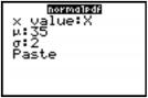
Note: For this example,
Xmin = 28
Xmax = 42
Xscl = 1
Ymin = 0
Ymax = .2
Yscl = .1
Note: For plotting the normal distribution, you can set window variables Xmin and Xmax so that the mean mu falls between them, and then select 0:ZoomFit from the ZOOM menu.
normalcdf(
normalcdf( computes the normal distribution probability between lowerbound and upperbound for the specified mean mu and standard deviation small sigma. The defaults are mu=0 and small sigma=1.
normalcdf(lowerbound,upperbound[,mu, small sigma])
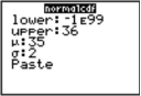
![]()
invNorm(
invNorm( computes the inverse cumulative normal distribution function for a given area under the normal distribution curve specified by mean mu and standard deviation small sigma. It calculates the x value associated with an area to the left of the x value. 0 less than or equal to area less than or equal to 1 must be true. The defaults are mu=0 and small sigma=1.
invNorm(area[,mu,small sigma])
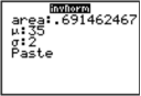
![]()
invT(
invT( computes the inverse cumulative Student-t probability function specified by Degree of Freedom, df for a given Area under the curve.
invT(area,df)
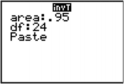
tpdf(
tpdf( computes the probability density function (pdf) for the Student-t distribution at a specified x value. df (degrees of freedom) must be greater than 0. To plot the Student-t distribution, paste tpdf( to the Y= editor. The probability density function (pdf) is:
fx ï‡ï›ï€¨df + 1/2ï
1 + x2
/df
–df + 1/2
= --------------------------------
ï‡ï€¨df  2
![]()
------------------------------------------------
ï°df
tpdf(x,df)
![]()
tcdf(
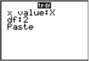
Note: For this example,
Xmin = -4.5
Xmax = 4.5
Ymin = 0
Ymax = .4
tcdf( computes the Student-t distribution probability between lowerbound and upperbound for the specified df (degrees of freedom), which must be greater than 0.
tcdf(lowerbound,upperbound,df)
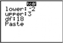
![]()
chi-square pdf(
chi-square pdf( computes the probability density function (pdf) for the chi-square distribution at a specified x value. df (degrees of freedom) must be an integer greater than 0. To plot the chi-square distribution, paste chi-square pdf( to the Y= editor. The probability density function (pdf) is:
fx =
---------1-----------1/2df/2xdf  2 – 1e–x/2,x  0
ï‡ï€¨df  2
chi-square pdf(x,df)
chi-square cdf(
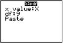
Note: For this example,
Xmin = 0
Xmax = 30
Ymin = -.02
Ymax = .132
chi-square cdf( computes the chi-square distribution probability between lowerbound and upperbound
for the specified df (degrees of freedom), which must be an integer greater than 0.
chi-square cdf(lowerbound,upperbound,df)
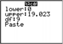
![]()
Fpdf(
Fpdf( computes the probability density function (pdf) for the F distribution at a specified x value. numerator df (degrees of freedom) and denominator df must be integers greater than 0. To plot the F distribution, paste Fpdf( to the Y= editor. The probability density function (pdf) is:
fx ï‡ï›ï€¨n + d/2ï  n  n/2
n/2 – 1
–n + d/2
= --------------------------------- --  x
1 + nx/d
,x  0
ï‡ï€¨n/2ï‡ï€¨ d/2 d
where n = numerator degrees of freedom
d = denominator degrees of freedom
Fpdf(x,numerator df,denominator df)
![]()
Fcdf(
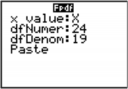
Note: For this example,
Xmin = 0
Xmax = 5
Ymin = 0
Ymax = 1
Fcdf( computes the F distribution probability between lowerbound and upperbound for the specified numerator df (degrees of freedom) and denominator df. numerator df and denominator df must be integers greater than 0.
Fcdf(lowerbound,upperbound,numerator df,denominator df)
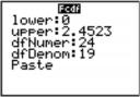
![]()
binompdf
binompdf( computes a probability at x for the discrete binomial distribution with the specified numtrials and probability of success (p) on each trial. x can be an integer or a list of integers. 0 less than or equal to p less than or equal to 1 must be true. numtrials must be an integer greater than 0. If you do not specify x, a list of probabilities from 0 to numtrials is returned. The probability density function (pdf) is:
fx
=  n px1 – pn – x,x =
x 
0,1,...,n
where n = numtrials
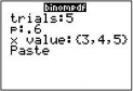
binompdf(numtrials,p[,x])
![]()
binomcdf(
binomcdf( computes a cumulative probability at x for the discrete binomial distribution with the specified numtrials and probability of success (p) on each trial. x can be a real number or a list of real numbers. 0 less than or equal to p less than or equal to 1 must be true. numtrials must be an integer greater than 0. If you do not specify x, a list of cumulative probabilities is returned.
binomcdf(numtrials,p[,x])
![]()
poissonpdf(
poissonpdf( computes a probability at x for the discrete Poisson distribution with the specified mean mu, which must be a real number greater than 0. x can be an integer or a list of integers. The probability density function (pdf) is:
fx
= e–ïïx  x!,x
= 0,1,2,...
poissonpdf(mu,x)
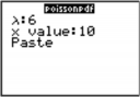
![]()
poissoncdf(
poissoncdf( computes a cumulative probability at x for the discrete Poisson distribution with the specified mean mu, which must be a real number greater than 0. x can be a real number or a list of real numbers.
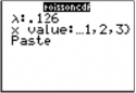
poissoncdf(mu,x)
![]()
geometpdf(
geometpdf( computes a probability at x, the number of the trial on which the first success occurs, for the discrete geometric distribution with the specified probability of success p. 0 less than or equal to p less than or equal to 1 must be true. x can be an integer or a list of integers. The probability density function (pdf) is:
fx
= p1 – px – 1,x =
1,2,...
geometpdf(p,x)
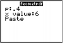
![]()
geometcdf(
geometcdf( computes a cumulative probability at x, the number of the trial on which the first success occurs, for the discrete geometric distribution with the specified probability of success p. 0 less than or equal to p less than or equal to 1 must be true. x can be a real number or a list of real numbers.
geometcdf(p,x)
![]()
![]()
MathPrintâ„¢ Classic 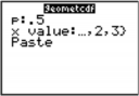
DISTR DRAW Menu
To display the DISTR DRAW menu, press [2nd] [DISTR][right key]. DISTR DRAW instructions draw various types of density functions, shade the area specified by lowerbound and upperbound, and display the computed area value.
Selecting an item from the DIST DRAW menu opens a wizard for the input of syntax for that item. Some of the arguments are optional. If an argument is not optional, the cursor will not move on to the next argument until a value is entered.
If you access any of these functions through CATALOG, the command or function will paste and you will be required to fill in the arguments.
To clear the drawings, select 1:ClrDraw from the DRAW menu (Chapter 8).
Note: Before you execute a DISTR DRAW instruction, you must set the window variables so that the desired distribution fits the screen.
![]()
DISTR DRAW
1: ShadeNorm( Shades normal distribution.
2: Shade_t( Shades Student-t distribution.
3: Shade chi- square
Shades chi-square distribution.
4: ShadeF Shades F distribution.
![]()
Note: -1E99 and 1E99 specify infinity. If you want to view the area left of upperbound, for example, specify lowerbound=-1E99.
ShadeNorm(
ShadeNorm( draws the normal density function specified by mean mu and standard deviation small sigma and shades the area between lowerbound and upperbound. The defaults are mu=0 and small sigma=1.
ShadeNorm(lowerbound,upperbound[,mu, small sigma])
![]()
Classic
Shade_t(
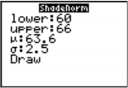
Note: For this example,
Xmin = 55
Xmax = 72
Ymin = -.05
Ymax = .2
Shade_t( draws the density function for the Student-t distribution specified by df (degrees of freedom) and shades the area between lowerbound and upperbound.
Shade_t(lowerbound,upperbound,df)
![]()
Classic
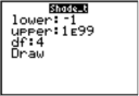
Note: For this example,
Xmin = -3
Xmax = 3
Ymin = -.15
Ymax = .5
Shade chi-square(
Shade chi-square( draws the density function for the chi-square distribution specified by df (degrees of freedom) and shades the area between lowerbound and upperbound.
Shade chi-square (lowerbound,upperbound,df)
![]()
Classic
ShadeF(
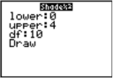
Note: For this example,
Xmin = 0
Xmax = 35
Ymin = -.025
Ymax = .1
ShadeF( draws the density function for the F distribution specified by numerator df (degrees of freedom) and denominator df and shades the area between lowerbound and upperbound.
ShadeF(lowerbound,upperbound,numerator df,denominator df)
![]()
Classic
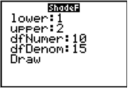
Note: For this example,
Xmin = 0
Xmax = 5
Ymin = -.25
Ymax = .9
The TI-84 Plus comes with several applications already installed and listed on the APPLICATIONS
menu. These applications include the following:
Finance
Topics in Algebra 1 Science Tools Catalog Help 1.1 CellSheetâ„¢ Conic Graphing Inequality Graphing
Transformation Graphing Vernier EasyDataâ„¢ DataMate
Polynomial Root Finder and Simultaneous Equation Solver StudyCardsâ„¢
LearningCheckâ„¢
Except for the Finance application, you can add and remove applications as space permits. The
Finance application is built into the TI-84 Plus code and cannot be deleted.
Many other applications in addition to the ones mentioned above, including language localization applications, are included on your TI-84 Plus. Press [APPS] to see the complete list of applications that came with your calculator.
You can download additional TI-84 Plus software applications from education.ti.com that allow you to customize your calculator’s functionality even further. The calculator reserves 1.54 M of space within ROM memory specifically for applications.
Guidebooks for applications are on the Texas Instruments Web site at: education.ti.com/guides.
Steps for Running the Finance Application
Follow these basic steps when using the Finance application.
Press [APPS] [ENTER] to select the Finance
application.
Select from list of functions.

Getting Started is a fast-paced introduction. Read the chapter for details.
You have found a car you would like to buy. You can afford payments of 250 per month for four years. The car costs 9,000. Your bank offers an interest rate of 5%. What will your payments be? Can you afford it?
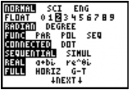
Press [MODE] [down key] [right key] [right key] [right key] [ENTER] to set the fixed-decimal mode setting to 2.

Press [APPS] [ENTER] to select 1:Finance from the
APPLICATIONS menu.
Press [ENTER] to select 1:TVM Solver from the
CALC VARS menu. The TVM Solver is displayed.
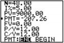
Enter the data:
N (number of payments)= 48
I% (interest rate)=5
PV (present value)=9000 FV (future value)=0
P/Y (payments per year)=12
C/Y (compounding periods per year)=12
Select PMT:END, which indicates that payments are due at the end of each period.
Move the cursor to PMT and press [ALPHA] [SOLVE].
Can you afford the payment?
At what annual interest rate, compounded monthly, will 1,250 accumulate to 2,000 in 7 years?
Note: Because there are no payments when you solve compound interest problems, PMT must be set to 0 and P/Y must be set to 1.
Press [APPS] [ENTER] to select 1:Finance from the
APPLICATIONS menu.
Press [ENTER] to select 1:TVM Solver from the CALC VARS menu. The TVM Solver is displayed.
Enter the data: N=7
PV=-1250 PMT=0
FV=2000 P/Y=1 C/Y=12
Move the cursor to I% and press [ALPHA] [SOLVE].
You need to look for an interest rate of 6.73% to grow 1250 to 2000 in 7 years.
Using the TVM Solver
The TVM Solver displays the time-value-of-money (TVM) variables. Given four variable values, the TVM Solver solves for the fifth variable.
The FINANCE VARS menu section describes the five TVM variables (N, I%, PV, PMT, and FV) and
P/Y and C/Y.
PMT: END BEGIN in the TVM Solver corresponds to the FINANCE CALC menu items Pmt_End
(payment at the end of each period) and Pmt_Bgn (payment at the beginning of each period). To solve for an unknown TVM variable, follow these steps.
Press [APPS] [ENTER] [ENTER] to display the TVM Solver. The screen below shows the default values with the fixed-decimal mode set to two decimal places.

Enter the known values for four TVM variables.
Note: Enter cash inflows as positive numbers and cash outflows as negative numbers.
Enter a value for P/Y, which automatically enters the same value for C/Y; if P/Y does not equal
C/Y, enter a unique value for C/Y.
Select END or BEGIN to specify the payment method.
Place the cursor on the TVM variable for which you want to solve.
Press [ALPHA] [SOLVE]. The answer is computed, displayed in the TVM Solver, and stored to the appropriate TVM variable. An indicator square in the left column designates the solution variable.
Entering Cash Inflows and Cash Outflows
When using the TI-84 Plus financial functions, you must enter cash inflows (cash received) as positive numbers and cash outflows (cash paid) as negative numbers. The TI-84 Plus follows this convention when computing and displaying answers.
FINANCE CALC Menu
To display the FINANCE CALC menu, press [APPS] [ENTER].
![]()
CALC VARS
1: TVM Solver... Displays the TVM Solver.
2: tvm_Pmt Computes the amount of each payment. 3: tvm_I% Computes the interest rate per year. 4: tvm_PV Computes the present value.
5: tvm_N Computes the number of payment periods.
6: tvm_FV Computes the future value.
7: npv( Computes the net present value.
![]()
![]()
CALC VARS
8: irr( Computes the internal rate of return.
9: bal( Computes the amortization sched. balance. 0: SigmaPrn( Computes the amort. sched. princ. sum. A: SigmaInt( Computes the amort. sched. interest sum. B: â–ºNom( Computes the nominal interest rate.
C: â–ºEff( Computes the effective interest rate. D: dbd( Calculates the days between two dates. E: Pmt_End Selects ordinary annuity (end of period).
F: Pmt_Bgn Selects annuity due (beginning of period).
![]()
Use these functions to set up and perform financial calculations on the home screen.
TVM Solver
TVM Solver displays the TVM Solver.
Calculating Time Value of Money
Use time-value-of-money (TVM) functions (menu items 2 through 6) to analyze financial instruments such as annuities, loans, mortgages, leases, and savings.
Each TVM function takes zero to six arguments, which must be real numbers. The values that you specify as arguments for TVM functions are not stored to the TVM variables.
Note: To store a value to a TVM variable, use the TVM Solver or use [STO right arrow] and any TVM
variable on the FINANCE VARS menu.
If you enter less than six arguments, the TI-84 Plus substitutes a previously stored TVM variable value for each unspecified argument.
If you enter any arguments with a TVM function, you must place the argument or arguments in parentheses.
tvm_Pmt
tvm_Pmt computes the amount of each payment.
tvm_Pmt[(N, I%,PV,FV,P/Y,C/Y)]
Note: In the example above, the values are stored to the TVM variables in the TVM Solver. The payment (tvm_Pmt) is computed on the home screen using the values in the TVM Solver. Next, the interest rate is changed to 9.5 to illustrate the effect on the payment amount.
tvm_I%
tvm_I% computes the annual interest rate.
tvm_I% [(N,PV,PMT,FV,P/Y,C/Y)]
MathPrintâ„¢ Classic
tvm_PV
tvm_PV computes the present value.
tvm_PV[(N, I%,PMT,FV,P/Y,C/Y)]
MathPrintâ„¢ Classic
tvm_N
tvm_N computes the number of payment periods.
tvm_N[(I%,PV,PMT,FV,P/Y,C/Y)]
MathPrintâ„¢ Classic
tvm_FV
tvm_FV computes the future value.
tvm_FV[(N, I%,PV,PMT,P/Y,C/Y)]
MathPrintâ„¢ Classic
Calculating a Cash Flow
Use the cash flow functions (menu items 7 and 8) to analyze the value of money over equal time periods. You can enter unequal cash flows, which can be cash inflows or outflows. The syntax descriptions for npv( and irr( use these arguments.
interest rate is the rate by which to discount the cash flows (the cost of money) over one period.
CF0 is the initial cash flow at time 0; it must be a real number.
CFList is a list of cash flow amounts after the initial cash flow CF0.
CFFreq is a list in which each element specifies the frequency of occurrence for a grouped (consecutive) cash flow amount, which is the corresponding element of CFList. The default is 1; if you enter values, they must be positive integers less than 10,000.
For example, express this uneven cash flow in lists.
2000
2000
2000
4000 4000
-3000
CF0 = 2000
CFList = {2000,-3000,4000}
CFFreq = {2,1,2}
npv(, irr(
npv( (net present value) is the sum of the present values for the cash inflows and outflows. A positive result for npv indicates a profitable investment.
npv(interest rate,CF0,CFList[,CFFreq])
irr( (internal rate of return) is the interest rate at which the net present value of the cash flows is equal to zero.
irr(CF0,CFList[,CFFreq])
1000
![]()
-2000 -2500
0 5000 3000
![]()
Calculating an Amortization Schedule
Use the amortization functions (menu items 9, 0, and A) to calculate balance, sum of principal, and sum of interest for an amortization schedule.
bal(
bal( computes the balance for an amortization schedule using stored values for I%, PV, and PMT. npmt is the number of the payment at which you want to calculate a balance. It must be a positive integer less than 10,000. roundvalue specifies the internal precision the calculator uses to calculate the balance; if you do not specify roundvalue, then the TI-84 Plus uses the current Float/Fix decimal- mode setting.
bal(npmt[,roundvalue])
Sigma Prn(, Sigma Int(
Sigma Prn( computes the sum of the principal during a specified period for an amortization schedule using stored values for I%, PV, and PMT. pmt1 is the starting payment. pmt2 is the ending payment in the range. pmt1 and pmt2 must be positive integers less than 10,000. roundvalue specifies the internal precision the calculator uses to calculate the principal; if you do not specify roundvalue, the TI-84 Plus uses the current Float/Fix decimal-mode setting.
Note: You must enter values for I%, PV, PMT, and before computing the principal.
Sigma Prn(pmt1,pmt2[,roundvalue])
Sigma Int( computes the sum of the interest during a specified period for an amortization schedule using stored values for I%, PV, and PMT. pmt1 is the starting payment. pmt2 is the ending payment in the range. pmt1 and pmt2 must be positive integers less than 10,000. roundvalue specifies the internal precision the calculator uses to calculate the interest; if you do not specify roundvalue, the
TI-84 Plus uses the current Float/Fix decimal-mode setting.
Sigma Int(pmt1,pmt2[,roundvalue])

Amortization Example: Calculating an Outstanding Loan Balance
You want to buy a home with a 30-year mortgage at 8 percent APR. Monthly payments are 800. Calculate the outstanding loan balance after each payment and display the results in a graph and in the table.
Press [MODE]. Press†[down key] [right key] [right key] [right key] [ENTER] to set the fixed-decimal mode setting to 2. Press [down key] [down key] [right key] [ENTER] to select Par graphing mode.
Press [APPS] [ENTER] [ENTER] to display the TVM Solver.
Press 360 to enter number of payments. Press [down key] 8 to enter the interest rate. Press [down key] [down key] [(-)] 800 to enter the payment amount. Press [down key] 0 to enter the future value of the mortgage. Press [down key] 12 to enter the payments per year, which also sets the compounding periods per year to 12. Press [down key] [down key] [ENTER] to select PMT:END.
Move the cursor to the PV prompt and then press
[ALPHA] [SOLVE] to solve for the present value.
![]()
Press [Y=] to display the parametric Y= editor. Turn off all stat plots. Press [X, T, theta, n] to define X1T as T. Press [down key] [APPS] [ENTER] 9 [X, T, theta, n] [)] to define Y1T as bal(T).
Press [WINDOW] to display the window variables.
Enter the values below.
|
Tmin=0 |
Xmin=0 |
Ymin=0 |
|
Tmax=360 |
Xmax=360 |
Ymax=125000 |
|
Tstep=12 |
Xscl=50 |
Yscl=10000 |
Press [TRACE] to draw the graph and activate the trace cursor. Press [right key] and [left key] to explore the graph of the outstanding balance over time. Press a number and then press [ENTER] to view the balance at a specific time T.
Press [2nd] [TBLSET] and enter the values below.
TblStart=0
Delta Tbl=12
Press [2nd] [TABLE] to display the table of outstanding balances (Y1T).
Press [MODE] and select G-T split-screen mode, so that the graph and table are displayed simultaneously.
Press [TRACE] to display X1T (time) and Y1T (balance) in the table.
Calculating an Interest Conversion
Use the interest conversion functions (menu items B and C) to convert interest rates from an annual effective rate to a nominal rate (â–ºNom( ) or from a nominal rate to an annual effective rate (â–ºEff( ).
â–ºNom(
â–ºNom( computes the nominal interest rate. effective rate and compounding periods must be real numbers. compounding periods must be greater than 0.
â–ºNom(effective rate,compounding periods)
![]()
â–ºEff(
â–ºEff( computes the effective interest rate. nominal rate and compounding periods must be real numbers. compounding periods must be greater than 0.
â–ºEff(nominal rate,compounding periods)
![]()
dbd(
Use the date function dbd( (menu item D) to calculate the number of days between two dates using the actual-day-count method. date1 and date2 can be numbers or lists of numbers within the range of the dates on the standard calendar.
Note: Dates must be between the years 1950 through 2049.
dbd(date1,date2)
You can enter date1 and date2 in either of two formats.
MM.DDYY (United States)
DDMM.YY (Europe)
The decimal placement differentiates the date formats.
![]()
MathPrintâ„¢
![]()
Classic
Defining the Payment Method
Pmt_End and Pmt_Bgn (menu items E and F) specify a transaction as an ordinary annuity or an annuity due. When you execute either command, the TVM Solver is updated.
Pmt_End
Pmt_End (payment end) specifies an ordinary annuity, where payments occur at the end of each payment period. Most loans are in this category. Pmt_End is the default.
Pmt_End
On the TVM Solver’s PMT:END BEGIN line, select END to set PMT to ordinary annuity.
Pmt_Bgn
Pmt_Bgn (payment beginning) specifies an annuity due, where payments occur at the beginning of each payment period. Most leases are in this category.
Pmt_Bgn
On the TVM Solver’s PMT:END BEGIN line, select BEGIN to set PMT to annuity due.
FINANCE VARS Menu
To display the FINANCE VARS menu, press [APPS] [ENTER] [right key]. You can use TVM variables in TVM functions and store values to them on the home screen.
![]()
CALC VARS
1: N Total number of payment periods
2: I% Annual interest rate
3: PV Present value
4: PMT Payment amount
5: FV Future value
6: P/Y Number of payment periods per year
![]()
![]()
CALC VARS
7: C/Y Number of compounding periods/year
![]()
N, I%, PV, PMT, FV
N, I%, PV, PMT, and FV are the five TVM variables. They represent the elements of common financial transactions, as described in the table above. I% is an annual interest rate that is converted to a per-period rate based on the values of P/Y and C/Y.
P/Y and C/Y
P/Y is the number of payment periods per year in a financial transaction.
C/Y is the number of compounding periods per year in the same transaction.
When you store a value to P/Y, the value for C/Y automatically changes to the same value. To store a unique value to C/Y, you must store the value to C/Y after you have stored a value to P/Y.
The Vernier EasyData™ application by Vernier Software & Technology allows you to view and analyze real-world data when the TI-84 Plus is connected to data collection devices such as Texas Instruments CBR 2™, CBL 2™, Vernier LabPro®, Vernier USB sensors, Vernier Go!™Motion, or Vernier Motion Detector Unit. The TI-84 Plus comes with the EasyData™ App already installed.
Note: The application will only work with Vernier auto-ID sensors when using CBL 2™ and Vernier LabPro®.
The EasyDataâ„¢ App will autolaunch on your TI-84 Plus if you plug in a USB sensor such as the CBR 2â„¢ or Vernier USB Temperature sensor.
Steps for Running the EasyDataâ„¢ App
Follow these basic steps when using the EasyDataâ„¢ App.
Starting the EasyDataâ„¢ App
Attach your data collection device to your TI-84 Plus.
Make sure the cables are firmly connected.
If the EasyDataâ„¢ App has not auto-launched, press [APPS] and the [up key] or [down key] to select the EasyDataâ„¢ App.
Press [ENTER]. The EasyDataâ„¢ information screen is displayed for about three seconds followed by the main screen.
Quitting the EasyDataâ„¢ App
To quit the EasyDataâ„¢ App, select Quit (press [GRAPH]).
The Ready to quit? screen is displayed, which indicates that the collected data has been transferred to lists L1 through L4 on the TI-84 Plus.
Press OK (press [GRAPH]) to quit.
EasyDataâ„¢ Settings
Changing EasyDataâ„¢ settings
The EasyDataâ„¢ App displays the most commonly used settings before data collection begins. To change a predefined setting:
From the main screen in the EasyDataâ„¢ App, choose Setup and select 2: Time Graph. The current settings are displayed on the calculator.
Note: If using a motion detector, settings for 3: Distance Match and 4: Ball Bounce in the Setup
menu are preset and cannot be changed.
Select Next (press [ZOOM]) to move to the setting you want to change. Press [CLEAR] to clear a setting.
Repeat to cycle through the available options. When the option is correct, select Next to move to the next option.
To change a setting, enter 1 or 2 digits, and then select Next (press [ZOOM]).
When all the settings are correct, select OK (press [GRAPH]) to return to the main menu.
Select Start (press [ZOOM]) to begin collecting data.
Restoring the EasyDataâ„¢ App to the default settings
The default settings are appropriate for a wide variety of sampling situations. If you are unsure of the best settings, begin with the default settings, and then adjust the settings for your specific activity.
To restore the default settings in the EasyDataâ„¢ App while a data collection device is connected to the TI-84 Plus, choose File and select 1:New.
Starting and Stopping Data Collection
Starting Data Collection
To start sampling, select Start (press [ZOOM]). Sampling will automatically stop when the number of samples set in the Time Graph Settings menu is reached. The TI-84 Plus will then display a graph of the sampled data.
Stopping Data Collection
To stop sampling before it automatically stops, select Stop (press and hold [ZOOM]) at any time during the sampling process. When sampling stops, a graph of the sampled data is displayed.
Saving Collected Data
Collected data is automatically transferred to the TI-84 Plus and stored in lists L1 through L4 when data collection is complete. When you exit the EasyDataâ„¢ App, a prompt reminds you of the lists in which time, distance, velocity, and acceleration are stored.
This manual describes basic operation for the EasyData 2 application. For more information about the EasyData 2 App, visit www.vernier.com.
What Is the CATALOG?
The CATALOG is an alphabetical list of all functions and instructions on the TI-84 Plus. You also can access each CATALOG item from a menu or the keyboard, except:
The six string functions
The six hyperbolic functions
The solve( instruction without the equation solver editor (Chapter 2)
The inferential stat functions without the inferential stat editors (Chapter 13)
Note: The only CATALOG programming commands you can execute from the home screen are
GetCalc(, Get(, and Send(.
Selecting an Item from the CATALOG
To select a CATALOG item, follow these steps.
Press [2nd] [CATALOG] to display the CATALOG.

The â–º (right-facing triangle) in the first column is the selection cursor.
Press [down key] or [up key] to scroll the CATALOG until the selection cursor points to the item you want.
To jump to the first item beginning with a particular letter, press that letter; alpha-lock is on.
Items that begin with a number are in alphabetical order according to the first letter after the number. For example, 2-PropZTest( is among the items that begin with the letter P.
Functions that appear as symbols, such as +, superscript -1, < (less than), and square root(, follow the last item that begins with Z. To jump to the first symbol, !, press [theta].
Press [ENTER] to paste the item to the current screen.
![]()
Note:
From the top of the CATALOG menu, press [up key] to move to the bottom. From the bottom, press [down key] to move to the top.
When your TI-84 Plus is in MathPrintâ„¢ mode, many functions will paste the MathPrintâ„¢ template on the home screen. For example, abs( pastes the absolute value template on the home screen instead of abs(.
![]()
![]()
MathPrintâ„¢ Classic
What Is a String?
A string is a sequence of characters that you enclose within quotation marks. On the TI-84 Plus, a string has two primary applications.
It defines text to be displayed in a program.
It accepts input from the keyboard in a program. Characters are the units that you combine to form a string.
Each number, letter, and space counts as one character.
Each instruction or function name, such as sin( or cos(, counts as one character; the TI-84 Plus interprets each instruction or function name as one character.
Entering a String
To enter a string on a blank line on the home screen or in a program, follow these steps.
Press [ALPHA] ["] to indicate the beginning of the string.
Enter the characters that comprise the string.
Use any combination of numbers, letters, function names, or instruction names to create the string.
To enter a blank space, press [ALPHA][space key].
To enter several alpha characters in a row, press [2nd] [A-LOCK] to activate alpha-lock.
Press [ALPHA] ["] to indicate the end of the string.
"string"
Press [ENTER]. On the home screen, the string is displayed on the next line without quotations.
An ellipsis (...) indicates that the string continues beyond the screen. To scroll to see the entire string, press [right key] and [left key].
![]()
Note: A string must be enclosed in quotation marks. The quotation marks do not count as string characters.
String Variables
The TI-84 Plus has 10 variables to which you can store strings. You can use string variables with string functions and instructions.
To display the VARS STRING menu, follow these steps.
Press [VARS] to display the VARS menu. Move the cursor to 7:String.
Press [ENTER] to display the STRING secondary menu.
Storing a String to a String Variable
To store a string to a string variable, follow these steps.
Press [ALPHA] ["], enter the string, and press [ALPHA]["].
Press [STO right arrow].
Press [VARS] 7 to display the VARS STRING menu.
Select the string variable (from Str1 to Str9, or Str0) to which you want to store the string.
The string variable is pasted to the current cursor location, next to the store symbol (right arrow).
Press [ENTER] to store the string to the string variable. On the home screen, the stored string is displayed on the next line without quotation marks.
![]()
Displaying the Contents of a String Variable
To display the contents of a string variable on the home screen, select the string variable from the
VARS STRING menu, and then press [ENTER]. The string is displayed.
![]()
Displaying String Functions and Instructions in the CATALOG
String functions and instructions are available only from the CATALOG. The table below lists the string functions and instructions in the order in which they appear among the other CATALOG menu items. The ellipses in the table indicate the presence of additional CATALOG items.
![]()
CATALOG
...
Equâ–ºString( Converts an equation to a string.
...
expr( Converts a string to an expression.
...
inString( Returns a character’s place number.
...
length( Returns a string’s character length.
...
Stringâ–ºEqu( Converts a string to an equation.
sub( Returns a string subset as a string.
...
![]()
Concatenation
To concatenate two or more strings, follow these steps.
Enter string1, which can be a string or string name.
Press [+].
Enter string2, which can be a string or string name. If necessary, press [+] and enter string3, and so on.
string1+string2+string3...
Press [ENTER] to display the strings as a single string.
Selecting a String Function from the CATALOG
To select a string function or instruction and paste it to the current screen, follow the steps for selecting an item from the CATALOG.
Equâ–ºString(
Equâ–ºString( converts an equation to a string. The equation must be store in a VARS Y-VARS variable. Yn contains the equation. Strn (from Str1 to Str9, or Str0) is the string variable to which you want the equation to be stored.
Equâ–ºString(Yn,Strn)
expr(
expr( converts the character string contained in string to an expression and executes it. string can be a string or a string variable.
expr(string)
inString(
inString( returns the character position in string of the first character of substring. string can be a string or a string variable. start is an optional character position at which to start the search; the default is 1.
inString(string,substring[,start])
Note: If string does not contain substring, or start is greater than the length of string, inString( returns 0.
length(
length( returns the number of characters in string. string can be a string or string variable. Note: An instruction or function name, such as sin( or cos(, counts as one character. length(string)
![]()
Stringâ–ºEqu(
Stringâ–ºEqu( converts string into an equation and stores the equation to Yn. string can be a string or string variable. Stringâ–ºEqu( is the inverse of Equâ–ºString(.
Stringâ–ºEqu(string,Yn)
![]()
sub(
sub( returns a string that is a subset of an existing string. string can be a string or a string variable. begin is the position number of the first character of the subset. length is the number of characters in the subset.
sub(string,begin,length)
![]()
Entering a Function to Graph during Program Execution
In a program, you can enter a function to graph during program execution using these commands.
![]()
Note: When you execute this program, enter a function to store to Y3 at the ENTRY= prompt.
Hyperbolic Functions
The hyperbolic functions are available only from the CATALOG. The table below lists the hyperbolic functions in the order in which they appear among the other CATALOG menu items. The ellipses in the table indicate the presence of additional CATALOG items.
![]()
CATALOG
...
cosh( Hyperbolic cosine
cosh superscript -1( Hyperbolic arccosine
...
sinh( Hyperbolic sine
sinh superscript -1( Hyperbolic arcsine
...
tanh( Hyperbolic tangent
tanh superscript -1( Hyperbolic arctangent
...
![]()
sinh(, cosh(, tanh(
sinh(, cosh(, and tanh( are the hyperbolic functions. Each is valid for real numbers, expressions, and lists.
sinh(value) cosh(value) tanh(value)
sinh superscript -1(, cosh superscript -1(, tanh superscript -1(
sinh superscript -1( is the hyperbolic arcsine function. cosh superscript -1( is the hyperbolic arccosine function. tanh superscript -1( is the hyperbolic arctangent function. Each is valid for real numbers, expressions, and lists.
sinh superscript -1(value) cosh superscript -1(value) tanh superscript -1(value)
![]()
Getting Started is a fast-paced introduction. Read the chapter for details.
A program is a set of commands that the TI-84 Plus executes sequentially, as if you had entered them from the keyboard. Create a program that prompts for the radius R and the height H of a cylinder and then computes its volume.
Press [PRGM] [right key] [right key] to display the
PRGM NEW menu.
Press [ENTER] to select 1:Create New. The Name= prompt is displayed, and alpha-lock is on. Press C Y L I N D E R, and then press [ENTER] to name the program CYLINDER.
You are now in the program editor. The colon (:) in the first column of the second line indicates the beginning of a command line.
Press [PRGM] [right key] 2 to select 2:Prompt from the PRGM I/O menu. Prompt is copied to the command line. Press [ALPHA] R [,][ALPHA] H to enter the variable names for radius and height. Press [ENTER].
Press [2nd] [pi] [ALPHA] R [x square][ALPHA] H [STO right arrow][ALPHA] V [ENTER] to enter the expression piR square H and store it to the variable V.
Press [PRGM] [right key] 3 to select 3:Disp from the PRGM I/O menu. Disp is pasted to the command line. Press [2nd] [A-LOCK] ["] V O L U M E [space key] I S ["] [ALPHA] [,] [ALPHA] V [ENTER] to set
up the program to display the text VOLUME IS on one line and the calculated value of V on the next.
Press [2nd] [QUIT] to display the home screen.

Press [PRGM] to display the PRGM EXEC menu.
The items on this menu are the names of stored programs.
Press [ENTER] to paste prgmCYLINDER to the current cursor location. (If CYLINDER is not item 1 on your PRGM EXEC menu, move the cursor to CYLINDER before you press [ENTER].)
Press [ENTER] to execute the program. Enter 1.5 for the radius, and then press [ENTER]. Enter 3 for the height, and then press [ENTER]. The text VOLUME IS, the value of V, and Done are displayed.
Repeat steps 7 through 9 and enter different values for R and H.
What Is a Program?
A program is a set of one or more command lines. Each line contains one or more instructions. When you execute a program, the TI-84 Plus performs each instruction on each command line in the same order in which you entered them. The number and size of programs that the TI-84 Plus can store is limited only by available memory.
Operating Systems versions and programming
Programs created with OS 2.43 and earlier should run correctly but may give unexpected results when you run them using OS 2.53MP and higher. You should test programs created with earlier OS versions to make sure you get the desired results.
Programs can run in Classic or MathPrintâ„¢ mode.
Shortcut menus are available wherever the MATH menu can be accessed.
MathPrintâ„¢ templates are not available for programs. All input and output is in Classic format.
You can use fractions in programs, but you should test the program to make sure that you get the desired results.
The spacing of the display may be slightly different in MathPrintâ„¢ mode than in Classic mode.
If you prefer the spacing in Classic mode, set the mode using a command in your program. Screen shots for the examples in this chapter were taken in Classic mode.
Stat Wizards are available only for syntax help for functions in the DISTR DISTR menu and the seq( function (sequence) in the LIST OPS menu. Run the Catalog Help application for more syntax help when programming.
Creating a New Program
To create a new program, follow these steps.
Press [PRGM] [left key] to display the PRGM NEW menu.
![]()
Press [ENTER] to select 1:Create New. The Name= prompt is displayed, and alpha-lock is on.
Press a letter from A to Z or theta to enter the first character of the new program name.
Note: A program name can be one to eight characters long. The first character must be a letter from A to Z or theta. The second through eighth characters can be letters, numbers, or theta.
Enter zero to seven letters, numbers, or theta to complete the new program name.
Press [ENTER]. The program editor is displayed.
Enter one or more program commands.
Press [2nd] [QUIT] to leave the program editor and return to the home screen.
Managing Memory and Deleting a Program
To check whether adequate memory is available for a program you want to enter:
Press [2nd] [MEM] to display the MEMORY menu.
Select 2:Mem Mgmt/Del to display the MEMORY MANAGEMENT/DELETE menu (Chapter 18).
Select 7:Prgm to display the PRGM editor.
The TI-84 Plus expresses memory quantities in bytes.
You can increase available memory in one of two ways. You can delete one or more programs or you can archive some programs.
To increase available memory by deleting a specific program:
Press [2nd] [MEM] and then select 2:Mem Mgmt/Del from the MEMORY menu.
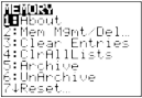
Select 7:Prgm to display the PRGM editor (Chapter 18).

Press [up key] and [down key] to move the selection cursor next to the program you want to delete, and then press [DEL]. The program is deleted from memory.
Note: You will receive a message asking you to confirm this delete action. Select 2:yes to continue.
To leave the PRGM editor screen without deleting anything, press [2nd] [QUIT], which displays the home screen.
To increase available memory by archiving a program:
Press [2nd] [MEM] and then select 2:Mem Mgmt/Del from the MEMORY menu.
Select 2:Mem Mgmt/Del to display the MEM MGMT/DEL menu.
Select 7:Prgm... to display the PRGM menu.
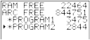
Press [ENTER] to archive the program. An asterisk will appear to the left of the program to indicate it is an archived program.
To unarchive a program in this screen, put the cursor next to the archived program and press
[ENTER]. The asterisk will disappear.
Note: Archive programs cannot be edited or executed. In order to edit or execute an archived program, you must first unarchive it.
Entering a Program Command Line
You can enter on a command line any instruction or expression that you could execute from the home screen. In the program editor, each new command line begins with a colon. To enter more than one instruction or expression on a single command line, separate each with a colon.
Note: A command line can be longer than the screen is wide.
While in the program editor, you can display and select from menus. You can return to the program editor from a menu in either of two ways.
Select a menu item, which pastes the item to the current command line.
— or —
Press [CLEAR].
When you complete a command line, press [ENTER]. The cursor moves to the next command line.
Programs can access variables, lists, matrices, and strings saved in memory. If a program stores a new value to a variable, list, matrix, or string, the program changes the value in memory during execution.
You can call another program as a subroutine.
Executing a Program
To execute a program, begin on a blank line on the home screen and follow these steps.
Press [PRGM] to display the PRGM EXEC menu.
Select a program name from the PRGM EXEC menu. prgmname is pasted to the home screen (for example, prgmCYLINDER).
Press [ENTER] to execute the program. While the program is executing, the busy indicator is on.
Last Answer (Ans) is updated during program execution. Last Entry is not updated as each command is executed (Chapter 1).
The TI-84 Plus checks for errors during program execution. It does not check for errors as you enter a program.
Breaking a Program
To stop program execution, press [ON]. The ERR:BREAK menu is displayed.
To return to the home screen, select 1:Quit.
To go where the interruption occurred, select 2:Goto.
Editing a Program
To edit a stored program, follow these steps.
Press [PRGM] [right key] to display the PRGM EDIT menu.
Select a program name from the PRGM EDIT menu. Up to the first seven lines of the program are displayed.
Note: The program editor does not display a $ to indicate that a program continues beyond the screen.
Edit the program command lines.
Move the cursor to the appropriate location, and then delete, overwrite, or insert.
Press [CLEAR] to clear all program commands on the command line (the leading colon remains), and then enter a new program command.
Note: To move the cursor to the beginning of a command line, press [2nd] [left key]; to move to the end, press [2nd] [right key]. To scroll the cursor down seven command lines, press [ALPHA] [down key]. To scroll the cursor up seven command lines, press [ALPHA] [up key].
Inserting and Deleting Command Lines
To insert a new command line anywhere in the program, place the cursor where you want the new line, press [2nd] [INS], and then press [ENTER]. A colon indicates a new line.
To delete a command line, place the cursor on the line, press [CLEAR] to clear all instructions and expressions on the line, and then press [DEL] to delete the command line, including the colon.
Copying and Renaming a Program
To copy all command lines from one program into a new program, follow steps 1 through 5 for Creating a New Program, and then follow these steps.
Press [2nd] [RCL]. Rcl is displayed on the bottom line of the program editor in the new program (Chapter 1).
Press [PRGM] [left key] to display the PRGM EXEC menu.
Select a name from the menu. prgmname is pasted to the bottom line of the program editor.
Press [ENTER]. All command lines from the selected program are copied into the new program.
Copying programs has at least two convenient applications.
You can create a template for groups of instructions that you use frequently.
You can rename a program by copying its contents into a new program.
Note: You also can copy all the command lines from one existing program to another existing program using RCL.
Scrolling the PRGM EXEC and PRGM EDIT Menus
The TI-84 Plus sorts PRGM EXEC and PRGM EDIT menu items automatically into alphanumerical order. Each menu only labels the first 10 items using 1 through 9, then 0.
To jump to the first program name that begins with a particular alpha character or theta, press
[ALPHA] [letter from A to Z or theta].
Note: From the top of either the PRGM EXEC or PRGM EDIT menu, press [up key] to move to the bottom. From the bottom, press [down key] to move to the top. To scroll the cursor down the menu seven items, press [ALPHA] [down key]. To scroll the cursor up the menu seven items, press [ALPHA] [up key].
PRGM CTL Menu
To display the PRGM CTL (program control) menu, press [PRGM] from the program editor only.
![]()
CTL I/O EXEC
|
1: |
If |
Creates a conditional test. |
|
2: |
Then |
Executes commands when If is true. |
|
3: |
Else |
Executes commands when If is false. |
|
4: |
For( |
Creates an incrementing loop. |
|
5: |
While |
Creates a conditional loop. |
|
6: |
Repeat |
Creates a conditional loop. |
|
7: |
End |
Signifies the end of a block. |
|
8: |
Pause |
Pauses program execution. |
|
9: |
Lbl |
Defines a label. |
|
0: |
Goto |
Goes to a label. |
|
A: |
IS>( |
Increments and skips if greater than. |
|
B: |
DS<( |
Decrements and skips if less than. |
|
C: |
Menu( |
Defines menu items and branches. |
|
D: |
prgm |
Executes a program as a subroutine. |
|
E: |
Return |
Returns from a subroutine. |
|
F: |
Stop |
Stops execution. |
|
G: |
DelVar |
Deletes a variable from within program. |
|
H: |
GraphStyle( |
Designates the graph style to be drawn. |
|
I: |
OpenLib( |
No longer used. |
|
J: |
ExecLib( |
No longer used. |
![]()
These menu items direct the flow of an executing program. They make it easy to repeat or skip a group of commands during program execution. When you select an item from the menu, the name is pasted to the cursor location on a command line in the program.
To return to the program editor without selecting an item, press [CLEAR].
Controlling Program Flow
Program control instructions tell the TI-84 Plus which command to execute next in a program. If, While, and Repeat check a defined condition to determine which command to execute next. Conditions frequently use relational or Boolean tests (Chapter 2), as in:
If A<7:A+1 right arrow A
or
If N=1 and M=1:Goto Z
If
Use If for testing and branching. If condition is false (zero), then the command immediately following If is skipped. If condition is true (nonzero), then the next command is executed. If instructions can be nested.
:If condition
:command (if true)
:command
Program Output
If-Then
Then following an If executes a group of commands if condition is true (nonzero). End identifies the end of the group of commands.
:If condition
:Then
:command (if true)
:command (if true)
:End
:command
Program Output

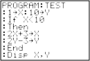
If-Then-Else
Else following If-Then executes a group of commands if condition is false (zero). End identifies the end of the group of commands.
:If condition
:Then
:command (if true)
:command (if true)
:Else
:command (if false)
:command (if false)
:End
:command
Program Output
![]()
![]()
Note: In OS 2.53MP and higher, the program name displays again when you press [ENTER] to repeat the program.
For(
For( loops and increments. It increments variable from begin to end by increment. increment is optional (default is 1) and can be negative (end less than begin). end is a maximum or minimum value not to be exceeded. End identifies the end of the loop. For( loops can be nested.
:For(variable,begin,end[,increment])
:command (while end not exceeded)
:command (while end not exceeded)
:End
:command
Program Output
While
While performs a group of commands while condition is true. condition is frequently a relational test (Chapter 2). condition is tested when While is encountered. If condition is true (nonzero), the program executes a group of commands. End signifies the end of the group. When condition is false (zero), the program executes each command following End. While instructions can be nested.
:While condition
:command (while condition is true)
:command (while condition is true)
:End
:command
Program Output
Repeat
Repeat repeats a group of commands until condition is true (nonzero). It is similar to While, but condition is tested when End is encountered; therefore, the group of commands is always executed at least once. Repeat instructions can be nested.
:Repeat condition
:command (until condition is true)
:command (until condition is true)
:End
:command
Program Output
End
End identifies the end of a group of commands. You must include an End instruction at the end of each For(, While, or Repeat loop. Also, you must paste an End instruction at the end of each If-Then group and each If-Then-Else group.
Pause
Pause suspends execution of the program so that you can see answers or graphs. During the pause, the pause indicator is on in the top-right corner. Press [ENTER] to resume execution.
Pause without a value temporarily pauses the program. If the DispGraph or Disp instruction has been executed, the appropriate screen is displayed.
Pause with value displays value on the current home screen. value can be scrolled.
Pause [value]
Program Output
![]()
![]()
Lbl, Goto
Lbl (label) and Goto (go to) are used together for branching.
Lbl specifies the label for a command. label can be one or two characters (A through Z, 0 through 99, or theta).
Lbl label
Goto causes the program to branch to label when Goto is encountered.
Goto label
Program Output
IS>(
IS>( (increment and skip) adds 1 to variable. If the answer is greater than value (which can be an expression), the next command is skipped; if the answer is less than or equal to value, the next command is executed. variable cannot be a system variable.
:IS>(variable,value)
:command (if answer is less than or equal to value)
:command (if answer is greater than value)
Program Output
Note: IS>( is not a looping instruction.
DS<(
DS<( (decrement and skip) subtracts 1 from variable. If the answer is less than value (which can be an expression), the next command is skipped; if the answer is greater than or equal to value, the next command is executed. variable cannot be a system variable.
:DS<(variable,value)
:command (if answer greater than or equal to value)
:command (if answer less than value)
Program Output
Note: DS<( is not a looping instruction.
Menu(
Menu( sets up branching within a program. If Menu( is encountered during program execution, the menu screen is displayed with the specified menu items, the pause indicator is on, and execution pauses until you select a menu item.
The menu title is enclosed in quotation marks ("). Up to seven pairs of menu items follow. Each pair comprises a text item (also enclosed in quotation marks) to be displayed as a menu selection, and a label item to which to branch if you select the corresponding menu selection.
Menu("title","text1",label1,"text2",label2, . . .) Program Output
The program above pauses until you select 1 or 2. If you select 2, for example, the menu disappears and the program continues execution at Lbl B.
prgm
Use prgm to execute other programs as subroutines. When you select prgm, it is pasted to the cursor location. Enter characters to spell a program name. Using prgm is equivalent to selecting existing programs from the PRGM EXEC menu; however, it allows you to enter the name of a program that you have not yet created.
prgmname
Note: You cannot directly enter the subroutine name when using RCL. You must paste the name from the PRGM EXEC menu.
Return
Return quits the subroutine and returns execution to the calling program, even if encountered within nested loops. Any loops are ended. An implied Return exists at the end of any program that is called as a subroutine. Within the main program, Return stops execution and returns to the home screen.
Stop
Stop stops execution of a program and returns to the home screen. Stop is optional at the end of a program.
DelVar
DelVar deletes from memory the contents of variable.
DelVar variable
![]()
GraphStyle(
GraphStyle( designates the style of the graph to be drawn. function# is the number of the Y= function name in the current graphing mode. graphstyle is a number from 1 to 7 that corresponds to the graph style, as shown below.
1 = line
2 = thick
3 = shade above
4 = shade below
5 = path
6 = animate
7 = dot
GraphStyle(function#,graphstyle)
For example, GraphStyle(1,5) in Func mode sets the graph style for Y1 to path; 5.
Not all graph styles are available in all graphing modes. For a detailed description of each graph style, see the Graph Styles table in Chapter 3.
PRGM I/O Menu
To display the PRGM I/O (program input/output) menu, press [PRGM] [right key] from within the program editor only.
![]()
CTL I/O EXEC
1: Input Enters a value or uses the cursor.
2: Prompt Prompts for entry of variable values. 3: Disp Displays text, value, or the home screen. 4: DispGraph Displays the current graph.
5: DispTable Displays the current table.
6: Output( Displays text at a specified position. 7: getKey Checks the keyboard for a keystroke. 8: ClrHome Clears the display.
9: ClrTable Clears the current table.
![]()
0: GetCalc( Gets a variable from another TI-84 Plus. A: Get( Gets a variable from CBL 2â„¢ or CBRâ„¢. B: Send( Sends a variable to CBL 2 or CBR.
These instructions control input to and output from a program during execution. They allow you to enter values and display answers during program execution.
To return to the program editor without selecting an item, press [CLEAR].
Displaying a Graph with Input
Input without a variable displays the current graph. You can move the free-moving cursor, which updates X and Y (and R and theta for PolarGC format). The pause indicator is on. Press [ENTER] to resume program execution.
Input
Program Output
![]()
![]()
Storing a Variable Value with Input
Input with variable displays a ? (question mark) prompt during execution. variable may be a real number, complex number, list, matrix, string, or Y= function. During program execution, enter a value, which can be an expression, and then press [ENTER]. The value is evaluated and stored to variable, and the program resumes execution.
Input [variable]
You can display text or the contents of Strn (a string variable) of up to 16 characters as a prompt. During program execution, enter a value after the prompt and then press [ENTER]. The value is stored to variable, and the program resumes execution.
Input ["text",variable]
Input [Strn,variable]
![]()
Program Output
![]()
Note: When a program prompts for input of lists and Yn functions during execution, you must include the braces ( { } ) around the list elements and quotation marks ( " ) around the expressions.
Prompt
During program execution, Prompt displays each variable, one at a time, followed by =?. At each prompt, enter a value or expression for each variable, and then press [ENTER]. The values are stored, and the program resumes execution.
Prompt variableA[,variableB,...,variable n]
Program Output
Note: Y= functions are not valid with Prompt.
Displaying the Home Screen
Disp (display) without a value displays the home screen. To view the home screen during program execution, follow the Disp instruction with a Pause instruction.
Disp
Displaying Values and Messages
Disp with one or more values displays the value of each.
Disp [valueA,valueB,valueC,...,value n]
If value is a variable, the current value is displayed.
If value is an expression, it is evaluated and the result is displayed on the right side of the next line.
If value is text within quotation marks, it is displayed on the left side of the current display line.
right arrow is not valid as text.
Program Output
![]()
![]()
If Pause is encountered after Disp, the program halts temporarily so you can examine the screen. To resume execution, press [ENTER].
Note: If a matrix or list is too large to display in its entirety, ellipses (...) are displayed in the last column, but the matrix or list cannot be scrolled. To scroll, use Pause value.
DispGraph
DispGraph (display graph) displays the current graph. If Pause is encountered after DispGraph, the program halts temporarily so you can examine the screen. Press [ENTER] to resume execution.
DispTable
DispTable (display table) displays the current table. The program halts temporarily so you can examine the screen. Press [ENTER] to resume execution.
Output(
Output( displays text or value on the current home screen beginning at row (1 through 8) and column
(1 through 16), overwriting any existing characters.
Note: You may want to precede Output( with ClrHome.
Expressions are evaluated and values are displayed according to the current mode settings. Matrices are displayed in entry format and wrap to the next line. right arrow is not valid as text.
Output(row,column,"text") Output(row,column,value)
Program Output
For Output( on a Horiz split screen, the maximum value for row is 4.
getKey
getKey returns a number corresponding to the last key pressed, according to the key code diagram below. If no key has been pressed, getKey returns 0. Use getKey inside loops to transfer control, for example, when creating video games.
Program Output
Note: [MATH], [APPS], [PRGM], and [ENTER]
![]()
were pressed during program execution.
Note: You can press [ON] any time during execution to break the program.
TI-84 Plus Key Code Diagram
ClrHome, ClrTable
ClrHome (clear home screen) clears the home screen during program execution.
ClrTable (clear table) clears the values in the table during program execution.
GetCalc(
GetCalc( gets the contents of variable on another TI-84 Plus and stores it to variable on the receiving TI-84 Plus. variable can be a real or complex number, list element, list name, matrix element, matrix name, string, Y= variable, graph database, or picture.
GetCalc(variable[,portflag])
By default, the TI-84 Plus uses the USB port if it is connected. If the USB cable is not connected, it uses the I/O port. If you want to specify either the USB or I/O port, use the following portflag numbers:
portflag=0 use USB port if connected;
portflag=1 use USB port;
portflag=2 use I/O port
Note: GetCalc( does not work between TI-82 and TI-83 Plus or a TI-82 and TI-84 Plus calculators.
Get(, Send(
Get( gets data from the CBL 2â„¢ or CBRâ„¢ and stores it to variable on the receiving TI-84 Plus. variable can be a real number, list element, list name, matrix element, matrix name, string, Y= variable, graph database, or picture.
Get(variable)
Note: If you transfer a program that references the Get( command to the TI-84 Plus from a TI-82, the TI-84 Plus will interpret it as the Get( described above. Use GetCalc( to get data from another TI-84 Plus.
Send( sends the contents of variable to the CBL 2â„¢ or CBRâ„¢. You cannot use it to send to another TI-84 Plus. variable can be a real number, list element, list name, matrix element, matrix name, string, Y= variable, graph database, or picture. variable can be a list of elements.
Send(variable)
Note: This program gets sound data and time in seconds from CBL 2â„¢.
Note: You can access Get(, Send(, and GetCalc( from the CATALOG to execute them from the home screen (Chapter 15).
Calling a Program from Another Program
On the TI-84 Plus, any stored program can be called from another program as a subroutine. Enter the name of the program to use as a subroutine on a line by itself.
You can enter a program name on a command line in either of two ways.
Press [PRGM] [left key] to display the PRGM EXEC menu and select the name of the program
prgmname is pasted to the current cursor location on a command line.
Select prgm from the PRGM CTL menu, and then enter the program name.
prgmname
When prgmname is encountered during execution, the next command that the program executes is the first command in the second program. It returns to the subsequent command in the first program when it encounters either Return or the implied Return at the end of the second program.
Program Output
![]()
Subroutine down arrow up arrow
![]()
Notes about Calling Programs
Variables are global.
label used with Goto and Lbl is local to the program where it is located. label in one program is not recognized by another program. You cannot use Goto to branch to a label in another program.
Return exits a subroutine and returns to the calling program, even if it is encountered within nested loops.
You can run programs written for the TI-84 Plus in assembly language. Typically, assembly language programs run much faster and provide greater control than the keystroke programs that you write with the built-in program editor.
Note: Because an assembly language program has greater control over the calculator, if your assembly language program has error(s), it may cause your calculator to reset and lose all data, programs, and applications stored in memory.
When you download an assembly language program, it is stored among the other programs as a
PRGM menu item. You can:
Transmit it using the TI-84 Plus communication link (Chapter 19).
Delete it using the MEM MGMT DEL screen (Chapter 18). To run an assembly Program, the syntax is: Asm( assemblyprgmname)
If you write an assembly language program, use the two instructions below from the CATALOG to identify and compile the program.
![]()
![]()
Instructions Comments
AsmComp(prgmASM1, prgmASM2)
Compiles an assembly language program written in ASCII and stores the hex version
![]()
AsmPrgm Identifies an assembly language program; must be entered as the first line of an assembly language program
![]()
To compile an assembly program that you have written:
Follow the steps for writing a program (16-4) but be sure to include AsmPrgm as the first line of your program.
From the home screen, press [2nd] [CATALOG] and then select AsmComp( to paste it to the screen.
Press [PRGM] to display the PRGM EXEC menu.
Select the program you want to compile. It will be pasted to the home screen.
Press [,] and then select prgm from the CATALOG.
Key in the name you have chosen for the output program.
Note: This name must be unique — not a copy of an existing program name.
Press [)] to complete the sequence.
The sequence of the arguments should be as follows:
AsmComp(prgmASM1, prgmASM2)
Press [ENTER] to compile your program and generate the output program.
Note: This example uses MathPrintâ„¢ mode for real answers and Classic mode for non-real (complex) results. You can also use the Polynomial Root Finder/Simultaneous Equation Solver application to solve these types of problems with a quick set-up. This application comes preloaded on your TI-84 Plus and can be downloaded from education.ti.com.
Use the quadratic formula to solve the quadratic equations 2x superscript 2 - 11x + 14 = 0 and 2x superscript 2 - 6x + 5 = 0.
Graphing the Functions
Before you begin, look at the graphs of the functions to see the approximate locations of the solutions.
Press [Y=] to display the Y= editor.
Press 2 [X, T, theta, n] [x square] [-]11 [X, T, theta, n] [+] 14 for Y1, and then press [ENTER].
Press 2 [X, T, theta, n] [x square] [-] 6 [X, T, theta, n] [+] 5 for Y2.
Press [ZOOM] and select 4:ZDecimal.
The graph of the functions displays.
You can see that the graph of the first function, 2x square - 11x + 14 = 0, crosses the x-axis, so it has a real solution. The graph of the second function does not cross the x-axis, so it has a complex solution.
Entering a Calculation
Begin with the equation 2x square - 11x + 14 = 0.
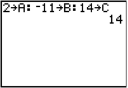
Press 2 [STO right arrow] [ALPHA] A to store the coefficient of the x square term.
Press [ALPHA] [:]. The colon allows you to enter more than one instruction on a line.
Press [(-)] 11 [STO right arrow] [ALPHA] B to store the coefficient of the X term. Press [ALPHA] [:] to enter a new instruction on the same line. Press 14 [STO right arrow] [ALPHA] C to store the constant.
Press [ENTER] to store the values to the variables A, B, and C.
The last value you stored is shown on the right side of the display. The cursor moves to the next line, ready for your next entry.
Press [ALPHA] [F1]1 [(-)] [ALPHA] B [+]
[2nd] [square root key] [ALPHA] B [x square]
[ -] 4 [ALPHA] A [ALPHA] C [right key] [right key] 2 [ALPHA] A to enter the expression for one of the solutions for the quadratic formula,
– b 
![]()
b2 – 4ac
--------------------------------------
2a
Press [ENTER] to find one solution for the equation 2x superscript 2 - 11x + 14 = 0.
The answer is shown on the right side of the display. The cursor moves to the next line, ready for you to enter the next expression.
Converting to a Decimal
You can show the solution as a decimal.
Press [ALPHA] [F1] 4 to select â–ºFâ—„â–º D
from the FRAC shortcut menu.
Press [ENTER] to convert the result to a decimal.
To save keystrokes, you can scroll up to find an expression you entered, copy it, and then edit it for a new calculation.
Press [up key] to highlight
![]() and then press [ENTER]
to paste it to the entry line.
and then press [ENTER]
to paste it to the entry line.
Press [left key] until the cursor is on the + sign in the formula. Press [-] to edit the quadratic-formula expression to become
![]() .
.
Press [ENTER] to find the other solution for the quadratic equation 2x square - 11x + 14 = 0.
Displaying Complex Results
Now solve the equation 2x square - 6x + 5 = 0. When you set a+bi complex number mode, the TI-84 Plus displays complex results.
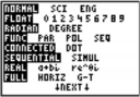
Press [MODE] [down key] [down key] [down key] [down key] [down key] [down key] (6 times), and then press [right key] to highlight a+bi. Press [ENTER] to select a+bi complex-number mode.
Press [2nd] [QUIT] to return to the home screen, and then press [CLEAR] to clear it.
Press 2 [STO right arrow] [ALPHA] A [ALPHA] [:] [(-)] 6 [STO right arrow] [ALPHA] B [ALPHA] [:] 5 [STO right arrow] [ALPHA] C [ENTER].
The coefficient of the x square term, the coefficient of the X term, and the constant for the new equation are stored to A, B, and C, respectively.
Enter the quadratic formula using Classic entry: [(] [(-)] [ALPHA] B [+] [2nd] [square root key] [ALPHA] B [x square] [-] 4 [ALPHA] A [ALPHA] C [right key] [)]
[division key] [(] 2 [ALPHA] A [)].
Because the solution is a complex number, you have to enter the formula using the division operation instead of using the n/d shortcut template. Complex numbers are not valid in the n/d template in input or output and will cause
Error: Data Type to display.
Press [ENTER] to find one solution for the equation 2x square - 6x + 5 = 0.
Press [up key] to highlight the quadratic- formula expression, and then press [ENTER] to paste it to the entry line.
Press [left key] until the cursor is on the + sign in the formula. Press [-] to edit the quadratic-formula expression to become
![]() .
.
Press [ENTER] to find the other solution for the quadratic equation: 2x square - 6x + 5 = 0.
Defining a Function
Take a 20 cm × 25 cm. sheet of paper and cut X × X squares from two corners. Cut X × 12½ cm rectangles from the other two corners as shown in the diagram below. Fold the paper into a box with a lid. What value of X would give your box the maximum volume V? Use the table and graphs to determine the solution.
Begin by defining a function that describes the volume of the box.
From the diagram: 2X + A = 20
2X + 2B = 25 V = A*B*X
Substituting:
V = (20 - 2X) (25/2 - X) X
X
20 A
X B X B 25

1. Press [Y=] to display the Y= editor, which is where you define functions for tables and graphing.
2. Press [(] 20 [-] 2 [X, T, theta, n] [)] [(] 25
[ALPHA] [F1] 1 2 [right key] [-] [X, T, theta,
n] [)] [X, T, theta, n] [ENTER] to define the volume function as Y1 in terms of X.
[X, T, theta, n] lets you enter X quickly, without having to press [ALPHA]. The highlighted = sign indicates that Y1 is selected.
Defining a Table of Values
The table feature of the TI-84 Plus displays numeric information about a function. You can use a table of values from the function you just defined to estimate an answer to the problem.
Press [2nd] [TBLSET] to display the
TABLE SETUP menu.
Press [ENTER] to accept TblStart=0.
Press 1 [ENTER] to define the table increment Delta Tbl=1. Leave Indpnt: Auto and Depend: Auto so that
the table will be generated automatically.
Press [2nd] [TABLE] to display the table.
Notice that the maximum value for Y1 (box’s volume) occurs when X is about 4, between 3 and 5.
Press and hold [down key] to scroll the table until a negative result for Y1 is displayed.
Notice that the maximum length of X for this problem occurs where the sign of Y1 (box’s volume) changes from positive to negative, between 10 and 11.
Press [2nd] [TBLSET].
Notice that TblStart has changed to 5 to reflect the first line of the table as it was last displayed. (In step 5, the first value of X displayed in the table is 5.)
Zooming In on the Table
You can adjust the way a table is displayed to get more information about a defined function. With smaller values for DeltaTbl, you can zoom in on the table. You can change the values on the TBLSET screen by pressing [2nd] [TBLSET] or by pressing [+] on the TABLE screen
Press [2nd] [TABLE].
Press [up key] to move the cursor to highlight 3.
Press [+]. The Delta Tbl displays on the entry line.
Enter [.] 1 [ENTER]. The table updates, showing the changes in X in increments of 0.1.
Notice that the maximum value for Y1 in this table view is 410.26, which occurs at X=3.7. Therefore, the maximum occurs where 3.6 less than X less than 3.8.
With X=3.6 highlighted, press [+] [.] 01
[ENTER] to set Delta Tbl=0.01.
Press [down key] and [up key] to scroll the table.
Four equivalent maximum values are shown, 410.26 at X=3.67, 3.68, 3.69, and
3.70.
Press [down key] or [up key] to move the cursor to 3.67. Press [right key] to move the cursor into the Y1 column.
The value of Y1 at X=3.67 is displayed on the bottom line in full precision as 410.261226.
Press [down key] to display the other maximum.
The value of Y1 at X=3.68 in full precision is 410.264064, at X=3.69 is 410.262318 and at X=3.7 is 410.256.
The maximum volume of the box would occur at 3.68 if you could measure and cut the paper at .01-centimeter increments.
Setting the Viewing Window
You also can use the graphing features of the TI-84 Plus to find the maximum value of a previously defined function. When the graph is activated, the viewing window defines the displayed portion of the coordinate plane. The values of the window variables determine the size of the viewing window.
Press [WINDOW] to display the window editor, where you can view and edit the values of the window variables.
The standard window variables define the viewing window as shown. Xmin, Xmax, Ymin, and Ymax define the boundaries of the display. Xscl and Yscl define the distance between tick marks on the X and Y axes. Xres controls resolution.
Press 0 [ENTER] to define Xmin.
Press 20 [division key] 2 to define Xmax
using an expression.
Note: For this example, the division sign is used for the calculation. However, you can use n/d entry format where fraction output can be experienced, depending on mode settings.
Press [ENTER]. The expression is evaluated, and 10 is stored in Xmax. Press [ENTER] to accept Xscl as 1.
Press 0 [ENTER] 500 [ENTER] 100
[ENTER] 1 [ENTER] to define the remaining window variables.
Displaying and Tracing the Graph
Now that you have defined the function to be graphed and the window in which to graph it, you can display and explore the graph. You can trace along a function using the TRACE feature.
Press [GRAPH] to graph the selected function in the viewing window.
The graph of Y1=(20-2X)(25/2-X)X is displayed.
Press [right key] to activate the free- moving graph cursor.
The X and Y coordinate values for the position of the graph cursor are displayed on the bottom line.
Press [left key], [right key], [up key], and [down key] to move the free-moving cursor to the apparent maximum of the function.
As you move the cursor, the X and Y coordinate values are updated continually.
Press [TRACE]. The trace cursor is displayed on the Y1 function.
The function that you are tracing is displayed in the top-left corner.
Press [left key] and [right key] to trace along Y1, one X dot at a time, evaluating Y1 at each X.
You also can enter your estimate for the maximum value of X.
Press 3 [.] 8. When you press a number key while in TRACE, the X= prompt is displayed in the bottom-left corner.
Press [ENTER].
The trace cursor jumps to the point on the Y1 function evaluated at X=3.8.
Press [left key] and [right key] until you are on the maximum Y value.
This is the maximum of Y1(X) for the X pixel values. The actual, precise maximum may lie between pixel values.
Zooming In on the Graph
To help identify maximums, minimums, roots, and intersections of functions, you can magnify the viewing window at a specific location using the ZOOM instructions.
Press [ZOOM] to display the ZOOM
menu.
This menu is a typical TI-84 Plus menu. To select an item, you can either press the number or letter next to the item, or you can press [down key] until the item number or letter is highlighted, and then press [ENTER].
Press 2 to select 2:Zoom In.
The graph is displayed again. The cursor has changed to indicate that you are using a ZOOM instruction.
With the cursor near the maximum value of the function, press [ENTER].
The new viewing window is displayed. Both Xmax-Xmin and Ymax-Ymin have been adjusted by factors of 4, the default values for the zoom factors.
Press [left key] and [right key] to search for the maximum value.
Press [WINDOW] to display the new window settings.
Note: To return to the previous graph, press [ZOOM] [right key] 1:ZPrevious.
Finding the Calculated Maximum
You can use a CALCULATE menu operation to calculate a local maximum of a function. To do this, pick a point to the left of where you think the maximum is on the graph. This is called the left bound. Next, pick a point to the right of the maximum. This is called the right bound. Finally, guess the maximum by moving the cursor to a point between the left and right bounds. With this information, the maximum can be calculated by the methods programmed in the TI-84 Plus.
Press [2nd] [CALC] to display the CALCULATE menu. Press 4 to select 4:maximum.
The graph is displayed again with a
Left Bound? prompt.
Press [left key] to trace along the curve to a point to the left of the maximum, and then press [ENTER].
A â–º at the top of the screen indicates the selected bound.
A Right Bound? prompt is displayed.
Press [right key] to trace along the curve to a point to the right of the maximum, and then press [ENTER].
A â—„ at the top of the screen indicates the selected bound.
A Guess? prompt is displayed.
Press [left key] to trace to a point near the maximum, and then press [ENTER].
Or, press 3 [.] 8, and then press [ENTER]
to enter a guess for the maximum.
When you press a number key in TRACE, the X= prompt is displayed in the bottom- left corner.
Notice how the values for the calculated maximum compare with the maximums found with the free-moving cursor, the trace cursor, and the table.
Note: In steps 2 and 3 above, you can enter values directly for Left Bound and Right Bound, in the same way as described in step 4.
Problem
An experiment found a significant difference between boys and girls pertaining to their ability to identify objects held in their left hands, which are controlled by the right side of their brains, versus their right hands, which are controlled by the left side of their brains. The TI Graphics team conducted a similar test for adult men and women.
The test involved 30 small objects, which participants were not allowed to see. First, they held 15 of the objects one by one in their left hands and guessed what they were. Then they held the other 15 objects one by one in their right hands and guessed what they were. Use box plots to compare visually the correct-guess data from this table.
Each row in the table represents the results observed for one subject. Note that 10 women and 12 men were tested.
|
Correct Guesses |
|||
|
Women Left |
Women Right |
Men Left |
Men Right |
|
8 |
4 |
7 |
12 |
|
9 |
1 |
8 |
6 |
|
12 |
8 |
7 |
12 |
|
11 |
12 |
5 |
12 |
|
10 |
11 |
7 |
7 |
|
8 |
11 |
8 |
11 |
|
12 |
13 |
11 |
12 |
|
7 |
12 |
4 |
8 |
|
9 |
11 |
10 |
12 |
|
11 |
12 |
14 |
11 |
|
13 |
9 |
||
|
5 |
9 |
||
Procedure
Press [STAT] 5 to select 5:SetUpEditor. Enter list names WLEFT, WRGHT, MLEFT, and MRGHT, separated by commas. Press [ENTER]. The stat list editor now contains only these four lists. (See Chapter 11: Lists for detailed instructions for using the SetUpEditor.)
Press [STAT] 1 to select 1:Edit.
Enter into WLEFT the number of correct guesses each woman made using her left hand (Women Left). Press [right key] to move to WRGHT and enter the number of correct guesses each woman made using her right hand (Women Right).
Likewise, enter each man’s correct guesses in MLEFT (Men Left) and MRGHT (Men Right).
Press [2nd] [STAT PLOT]. Select 1:Plot1. Turn on plot 1; define it as a modified box plot that uses Xlist as WLEFT. Move the cursor to the top line and select Plot2. Turn on plot 2; define it as a modified box plot that uses Xlist as WRGHT. (See Chapter 12: Statistics for detailed information on using Stat Plots.)
Press [Y=]. Turn off all functions.
Press [WINDOW]. Set Xscl=1 and Yscl=0. Press [ZOOM] 9 to select 9:ZoomStat. This adjusts the viewing window and displays the box plots for the women’s results.
Press [TRACE].
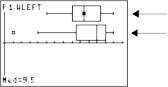
Women’s left-hand data Women’s right-hand data
Use [left key] and [right key] to examine minX, Q1, Med, Q3, and maxX for each plot. Notice the outlier to the women’s right-hand data. What is the median for the left hand? For the right hand? With which hand were the women more accurate guessers, according to the box plots?
Examine the men’s results. Redefine plot 1 to use MLEFT, redefine plot 2 to use MRGHT. Press
[TRACE].
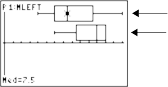
Men’s left-hand data Men’s right-hand data
Press [left key] and [right key] to examine minX, Q1, Med, Q3, and maxX for each plot. What difference do you see between the plots?
Compare the left-hand results. Redefine plot 1 to use WLEFT, redefine plot 2 to use MLEFT, and then press [TRACE] to examine minX, Q1, Med, Q3, and maxX for each plot. Who were the better left-hand guessers, men or women?
Compare the right-hand results. Define plot 1 to use WRGHT, define plot 2 to use MRGHT, and then press [TRACE] to examine minX, Q1, Med, Q3, and maxX for each plot. Who were the better right-hand guessers?
In the original experiment boys did not guess as well with right hands, while girls guessed equally well with either hand. This is not what our box plots show for adults. Do you think that this is because adults have learned to adapt or because our sample was not large enough?
Problem
The fine for speeding on a road with a speed limit of 45 kilometers per hour (kph) is 50; plus 5 for each kph from 46 to 55 kph; plus 10 for each kph from 56 to 65 kph; plus 20 for each kph from 66 kph and above. Graph the piecewise function that describes the cost of the ticket.
The fine (Y) as a function of kilometers per hour (X) is:
 ,
,
which simplifies to:
Procedure
Press [MODE]. Select Func and Classic.
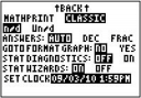
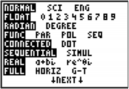
Press [Y=]. Turn off all functions and stat plots. Enter the Y= function to describe the fine. Use the TEST menu operations to define the piecewise function. Set the graph style for Y1 to dot.
Press [WINDOW] and set Xmin=-2, Xscl=10, Ymin=-5, Yscl=10 and Delta X=1. Ignore Xmax and
Ymax; they are set in step 4.
Press [2nd] [QUIT] to return to the home screen. Store 5 to DeltaY. DeltaX and DeltaY are on the VARS Window X/Y secondary menu. DeltaX and DeltaY specify the horizontal and vertical distance between the centers of adjacent pixels. Integer values for DeltaX and DeltaY produce nice values for tracing.
Press [TRACE] to plot the function. At what speed does the ticket exceed 250?
Problem
Graph the inequality 0.4x cube - 3x + 5 less than 0.2x + 4. Use the TEST menu operations to explore the values of X where the inequality is true and where it is false.
Note: You can also investigate graphing inequalities using the Inequality Graphing application. The application is pre-loaded on your TI-84 Plus and can be downloaded from education.ti.com.
Procedure
Press [MODE]. Select Dot, Simul, and the default settings. Setting Dot mode changes all graph style icons to dot in the Y= editor.
Press Y=. Turn off all functions and stat plots. Enter the left side of the inequality as Y4 and the right side as Y5.
Enter the statement of the inequality as Y6. This function evaluates to 1 if true or 0 if false.
Note: You can use the YVARS shortcut menu to paste Y4 and Y5 in the Y= editor.
Press [ZOOM] 6 to graph the inequality in the standard window.
Press [TRACE] [down key] [down key] to move to Y6. Then press [left key] and [right key] to trace the inequality, observing the value of Y.
When you trace, you can see that Y=1 indicates that Y4 less than Y5 is true and that Y=0 indicates that Y4 less than Y5 is false.
Press [Y=]. Turn off Y4, Y5, and Y6. Enter equations to graph only the inequality.
Press [TRACE].
Notice that the values of Y7 and Y8 are zero where the inequality is false. You only see the intervals of the graph where Y4 less than Y5 because intervals that are false are multiplied by 0 (Y6*Y4 and Y6*Y5)
Problem
Using a graph, solve the equation x cube - 2x=2cos(x). Stated another way, solve the system of two equations and two unknowns: y = x cube - 2x and y= 2cos(x). Use ZOOM factors to control the decimal places displayed on the graph and use [2nd] [CALC] 5:intersect to find an approximate solution.
Procedure
Press [MODE]. Select the default mode settings. Press [Y=]. Turn off all functions and stat plots.
Enter the functions.
![]()
Press [ZOOM] 4 to select 4:ZDecimal. The display shows that two solutions may exist (points where the two functions appear to intersect).
Press [ZOOM] [right key] 4 to select 4:SetFactors from the ZOOM MEMORY menu. Set XFact=10
and YFact=10.
Press [ZOOM] 2 to select 2:Zoom In. Use [left key], [right key], [up key], and [down key] to move the free-moving cursor onto the apparent intersection of the functions on the right side of the display. As you move the cursor, notice that the X and Y values have one decimal place.
Press [ENTER] to zoom in. Move the cursor over the intersection. As you move the cursor, notice that now the X and Y values have two decimal places.
Press [ENTER] to zoom in again. Move the free-moving cursor onto a point exactly on the intersection. Notice the number of decimal places.
Press [2nd][CALC] 5 to select 5:intersect. Press [ENTER] to select the first curve and [ENTER] to select the second curve. To guess, move the trace cursor near the intersection. Press [ENTER]. What are the coordinates of the intersection point?
Press [ZOOM] 4 to select 4:ZDecimal to redisplay the original graph.
Press [ZOOM]. Select 2:Zoom In and repeat steps 4 through 8 to explore the apparent function intersection on the left side of the display.
Setting up the Program
This program creates a drawing of a famous fractal, the Sierpinski Triangle, and stores the drawing to a picture. To begin, press [PRGM] [right key] [right key] 1. Name the program SIERPINS, and then press [ENTER]. The program editor is displayed.
Note: After you run this program, press [2nd] [FORMAT] [down key] [down key] [down key] [ENTER]
to turn on the axes in the graph screen.
Program
PROGRAM:SIERPINS
:FnOff :ClrDraw
:PlotsOff
:AxesOff
:0 right arrow Xmin:1right arrow Xmax
:0 right arrow Ymin:1 right arrow Ymax
:rand right arrow X:rand right arrow Y
![]()
Set viewing window.
:For(K,1,3000)
:rand right arrow N
:If N less than or equal to 1/ 3
:Then
:.5X right arrow X
:.5Y right arrow Y
:End
:If 1 /3 is less than N and N is less than or equal to 2 /3
:Then
:.5(.5+X)right arrow X
:.5(1+Y)right arrow Y
:End
:If 2 /3 i s le ss t han N
:Then
:.5(1+X)right arrow X
:.5Y right arrow Y
:End
:Pt-On(X,Y)
:End
:StorePic 6
![]() Beginning of For group.
Beginning of For group.
![]() If/Then group
If/Then group
![]() If/Then group.
If/Then group.
![]() If/Then group.
If/Then group.
Draw point.
End of For group. Store picture.
After you execute the program above, you can recall and display the picture with the instruction
RecallPic 6.

Problem
Using Web format, you can identify points with attracting and repelling behavior in sequence graphing.
Procedure
Press [MODE]. Select Seq and the default mode settings. Press [2nd] [FORMAT]. Select Web
format and the default format settings.
Press [Y=]. Clear all functions and turn off all stat plots. Enter the sequence that corresponds to the expression Y = K X(1 - X).
u(n)=Ku(n - 1)(1 - u(n - 1))
u(nMin)=.01
Press [2nd] [QUIT] to return to the home screen, and then store 2.9 to K.
Press [WINDOW]. Set the window variables.
nMin=0 nMax=10 PlotStart=1 PlotStep=1
Xmin=0 Xmax=1 Xscl=1
Ymin=-.26 Ymax=1.1 Yscl=1
Press [TRACE] to display the graph, and then press [right key] to trace the cobweb. This is a cobweb with one attractor.
Change K to 3.44 and trace the graph to show a cobweb with two attractors.
Change K to 3.54 and trace the graph to show a cobweb with four attractors.
Setting Up the Program
This program graphs the function A sin(BX) with random integer coefficients between 1 and 10. Try to guess the coefficients and graph your guess as C sin(DX). The program continues until your guess is correct.
Note: This program changes the graph window and graph styles. After you run the program, you can change individual settings as needed or you can press [2nd] [MEM] 7 2 2 to return to default settings.
Programs typically do not restore your settings in MODE, Y=, WINDOW and other locations that were used by the program. This is dependent on who created the program.
Program
PROGRAM:GUESS
:PlotsOff :Func
:FnOff :Radian
:ClrHome
:"Asin(BX)" right arrow Y1
![]()
:"Csin(DX)" right arrow Y2
Define equations.
:GraphStyle(1,1)
:GraphStyle(2,5)
![]()
Set line and path graph styles.
:FnOff 2
![]()
:randInt(1,10) right arrow A
:randInt(1,10) right arrow B
:0 right arrow C:0 right arrow
D
![]()
:-2pi right arrow Xmin
:2pi right arrow Xmax
:pi/2 right arrow Xscl
:-10 right arrow Ymin
:10 right arrow Ymax
:1 right arrow Yscl
![]()
:DispGraph
Initialize coefficients.
Set viewing window.
:Pause Display graph.
:FnOn 2
:Lbl Z
:Prompt C,D Prompt for guess.
![]()
:DispGraph
:Pause Display graph.
![]()
:If C=A
:Text(1,1,"C IS OK")
:If C is not equal to A
:Text(1,1,"C IS WRONG")
:If D=B
:Text(1,50,"D IS OK")
:If D is not equal to B
:Text(1,50,"D IS WRONG")
![]()
:DispGraph
Display results.
:Pause Display graph.
:If C=A and D=B
:Stop
:Goto Z
![]()
Quit if guesses are correct.
Note: The Guess My Coefficients App is an educational game that challenges you to enter the correct coeffiecients for graphs of linear, quadratic and absolute value functions. This app is available at education.ti.com.
Problem
Using parametric graphing mode, graph the unit circle and the sine curve to show the relationship between them.
Any function that can be plotted in Func mode can be plotted in Par mode by defining the X
component as T and the Y component as F(T).
Procedure
Press [MODE]. Select Par, Simul, and the default settings.
Press [WINDOW]. Set the viewing window.
Tmin=0 Tmax=2pi Tstep=.1
Xmin=-2 Xmax=7.4 Xscl=pi/2
Ymin=-3 Ymax=3 Yscl=1
Press [Y=]. Turn off all functions and stat plots. Enter the expressions to define the unit circle centered on (0,0).

Enter the expressions to define the sine curve.
Press [TRACE]. As the graph is plotting, you may press [ENTER] to pause and [ENTER] again to resume graphing as you watch the sine function “unwrap†from the unit circle.
Note:
You can generalize the unwrapping. Replace sin(T) in Y2T with any other trig function to unwrap that function.
You can graph the functions again by turning the functions off and then turning them back on on the Y= editor or by using the FuncOFF and FuncON commands on the home screen.
Problem
Find the area of the region bounded by:
f(x)
g(x) x
= 300x / (x square + 625)
= 3cos(.1x)
= 75
Procedure
Press [MODE]. Select the default mode settings.
Press [WINDOW]. Set the viewing window.
Xmin=0 Xmax=100 Xscl=10
Ymin=-5 Ymax=10 Yscl=1
Xres=1
Press [Y=]. Turn off all functions and stat plots. Enter the upper and lower functions.
Y1=300X/(X square+625) Y2=3cos(.1X)
Press [2nd] [CALC] 5 to select 5:Intersect. The graph is displayed. Select a first curve, second curve, and guess for the intersection toward the left side of the display. The solution is displayed, and the value of X at the intersection, which is the lower limit of the integral, is stored in Ans and X.
Press [2nd] [QUIT] to go to the home screen. Press [2nd] [DRAW] 7 and use Shade( to see the area graphically.
Shade(Y2,Y1,Ans,75)
Press [2nd] [QUIT] to return to the home screen. Enter the expression to evaluate the integral for the shaded region.
fnInt(Y1-Y2,X,Ans,75)
The area is 325.839962.
Problem
Using two pairs of parametric equations, determine when two objects in motion are closest to each other in the same plane.
A ferris wheel has a diameter (d) of 20 meters and is rotating counterclockwise at a rate (s) of one revolution every 12 seconds. The parametric equations below describe the location of a ferris wheel passenger at time T, where alpha is the angle of rotation, (0,0) is the bottom center of the ferris wheel, and (10,10) is the passenger’s location at the rightmost point, when T=0.
X(T) = r cos alpha
Y(T) = r + r sin alpha
where alpha = 2piTs and r = d /2
A person standing on the ground throws a ball to the ferris wheel passenger. The thrower’s arm is at the same height as the bottom of the ferris wheel, but 25 meters (b) to the right of the ferris wheel’s lowest point (25,0). The person throws the ball with velocity (v subscript 0) of 22 meters per second at an angle (theta) of 66° from the horizontal. The parametric equations below describe the location of the ball at time T.
X(T) = b - Tv subscript 0 cos theta
Y(T) = Tv subscript 0 sin theta - (g /2) T square where g = 9.8 m /sec square
Procedure
Press [MODE]. Select Par, Simul, and the default settings. Simul (simultaneous) mode simulates the two objects in motion over time.
Press [WINDOW]. Set the viewing window.
Tmin=0 Tmax=12 Tstep=.1
Xmin=-13 Xmax=34 Xscl=10
Ymin=0 Ymax=31 Yscl=10
Press [Y=]. Turn off all functions and stat plots. Enter the expressions to define the path of the ferris wheel and the path of the ball. Set the graph style for X2T to path.
![]()
Note: Try setting the graph styles to path X1T and animate X2T, which simulates a chair on the ferris wheel and the ball flying through the air when you press [GRAPH].
Press [GRAPH] to graph the equations. Watch closely as they are plotted. Notice that the ball and the ferris wheel passenger appear to be closest where the paths cross in the top-right quadrant of the ferris wheel.
Press [WINDOW]. Change the viewing window to concentrate on this portion of the graph.
Tmin=1 Tmax=3 Tstep=.03
Xmin=0 Xmax=23.5 Xscl=10
Ymin=10 Ymax=25.5 Yscl=10
Press [TRACE]. After the graph is plotted, press [right key] to move near the point on the ferris wheel where the paths cross. Notice the values of X, Y, and T.
Press [down key] to move to the path of the ball. Notice the values of X and Y (T is unchanged).
Notice where the cursor is located. This is the position of the ball when the ferris wheel passenger passes the intersection. Did the ball or the passenger reach the intersection first?
You can use [TRACE] to, in effect, take snapshots in time and explore the relative behavior of two objects in motion.
Problem 1
Using the functions fnInt( and nDeriv( from the FUNC shortcut menu or the MATH menu to graph functions defined by integrals and derivatives demonstrates graphically that:
![]() and that
and that
![]()
Procedure 1
Press [MODE]. Select the default settings.
Press [WINDOW]. Set the viewing window.
Xmin=.01 Xmax=10 Xscl=1
Ymin=-1.5 Ymax=2.5 Yscl=1
Xres=3
Press [Y=]. Turn off all functions and stat plots. Enter the numerical integral of 1/T from 1 to X and the function ln(X). Set the graph style for Y1 to line and Y2 to path.
Press [TRACE]. Press [left key], [up key], [right key], and [down key] to compare the values of
Y1 and Y2.
Press [Y=]. Turn off Y1 and Y2, and then enter the numerical derivative of the integral of 1/X and the function 1/X. Set the graph style for Y3 to line and Y4 to thick.
Press [TRACE]. Again, use the cursor keys to compare the values of the two graphed functions, Y3 and Y4.
Problem 2
Explore the functions defined by
x
y = 
t2dt,
x
 t2dt , and
x
 t2dt
–2 0 2
Procedure 2
Press [Y=]. Turn off all functions and stat plots. Use a list to define these three functions simultaneously. Store the function in Y5.
Press [ZOOM] 6 to select 6:ZStandard. The graphs are displayed as each calculation of the integral and derivative occurs at the pixel point, which may take some time.
Press [TRACE]. Notice that the functions appear identical, only shifted vertically by a constant.
Press [Y=]. Enter the numerical derivative of Y5 in Y6.
Press [TRACE]. Notice that although the three graphs defined by Y5 are different, they share the same derivative.
Problem
Use the equation solver to store a formula for the area of a regular N-sided polygon, and then solve for each variable, given the other variables. Explore the fact that the limiting case is the area
of a circle, pi r square.
Consider the formula A = NB square sin(pi/N) cos (pi/N) for the area of a regular polygon with N sides of equal length and B distance from the center to a vertex.
N = 4 sides N = 8 sides N = 12 sides
Procedure
Press [MATH] [ALPHA] B to select B:Solver from the MATH menu. Either the equation editor or the interactive solver editor is displayed. If the interactive solver editor is displayed, press [up key] to display the equation editor.
Enter the formula as 0=A-NB square sin (pi/N) cos (pi/N), and then press [ENTER]. The interactive solver editor is displayed.
Enter N=4 and B=6 to find the area (A) of a square with a distance (B) from center to vertex of 6 centimeters.
Press [up key][up key] to move the cursor onto A, and then press [ALPHA] [SOLVE]. The solution for A is displayed on the interactive solver editor.
Now solve for B for a given area with various number of sides. Enter A=200 and N=6. To find the distance B, move the cursor onto B, and then press [ALPHA] [SOLVE].
Enter N=8. To find the distance B, move the cursor onto B, and then press [ALPHA] [SOLVE].
Find B for N=9, and then for N=10.
Find the area given B=6, and N=10, 100, 150, 1000, and 10000. Compare your results with pi 6 square (the area of a circle with radius 6), which is approximately 113.097.
Enter B=6. To find the area A, move the cursor onto A, and then press [ALPHA] [SOLVE]. Find A for N=10, then N=100, then N=150, then N=1000, and finally N=10000. Notice that as N gets large, the area A approaches pi B square.
Now graph the equation to see visually how the area changes as the number of sides gets large.
Press [MODE]. Select the default mode settings.
Press [WINDOW]. Set the viewing window.
Xmin=0 Xmax=200 Xscl=10
Ymin=0 Ymax=150 Yscl=10
Xres=1
Press [Y=]. Turn off all functions and stat plots. Enter the equation for the area. Use X in place of N. Set the graph styles as shown.
Press [TRACE]. After the graph is plotted, press 100 [ENTER] to trace to X=100. Press 150 [ENTER]. Press 188 [ENTER]. Notice that as X increases, the value of Y converges to pi 6 square, which is approximately 113.097. Y2=pi B square(the area of the circle) is a horizontal asymptote to Y1. The area of an N-sided regular polygon, with r as the distance from the center to a vertex, approaches the area of a circle with radius r (pi r square) as N gets large.
Problem
You are a loan officer at a mortgage company, and you recently closed on a 30-year home mortgage at 8 percent interest with monthly payments of 800. The new home owners want to know how much will be applied to the interest and how much will be applied to the principal when they make the 240th payment 20 years from now.
Procedure
Press [MODE] and set the fixed-decimal mode to 2 decimal places. Set the other mode settings to the defaults.
Press [APPS] [ENTER] [ENTER] to display the TVM Solver. Enter these values.
Note: Enter a positive number (800) to show PMT as a cash inflow. Payment values will be displayed as positive numbers on the graph. Enter 0 for FV, since the future value of a loan is 0 once it is paid in full. Enter PMT: END, since payment is due at the end of a period.
Move the cursor onto the PV= prompt, and then press [ALPHA] [SOLVE]. The present value, or mortgage amount, of the house is displayed at the PV= prompt.
Now compare the graph of the amount of interest with the graph of the amount of principal for each payment.
Press [MODE]. Set Par and Simul.
Press [Y=]. Turn off all functions and stat plots. Enter these equations and set the graph styles as shown.
Note: Sigma Prn( and Sigma Int( are located on the FINANCE menu (APPS 1:FINANCE).
Press [WINDOW]. Set these window variables.
Tmin=1 Tmax=360 Tstep=12
Xmin=0 Xmax=360 Xscl=10
Ymin=0 Ymax=1000 Yscl=100
Note: To increase the graph speed, change Tstep to 24.
Press [TRACE]. After the graph is drawn, press 240 [ENTER] to move the trace cursor to
T=240, which is equivalent to 20 years of payments.
The graph shows that for the 240th payment (X=240), 358.03 of the 800 payment is applied to principal (Y=358.03).
Note: The sum of the payments (Y3T=Y1T+Y2T) is always 800.
Press [down key] to move the cursor onto the function for interest defined by X2T and Y2T. Enter 240.
The graph shows that for the 240th payment (X=240), 441.97 of the 800 payment is interest (Y=441.97).
Press [2nd] [QUIT][APPS] [ENTER] 9 to paste 9:bal( to the home screen. Check the figures from the graph.
At which monthly payment will the principal allocation surpass the interest allocation?
MEMORY Menu
At any time you can check available memory or manage existing memory by selecting items from the MEMORY menu. To access this menu, press [2nd] [MEM].
![]()
MEMORY
1: About... Displays information about the graphing
calculator including current OS version number.
2: Mem Mgmt/Del... Reports memory availability and variable usage.
3: Clear Entries Clears ENTRY (last-entry storage).
4: ClrAllLists Clears all lists in memory.
5: Archive... Archives a selected variable.
6: UnArchive... UnArchives a selected variable.
7: Reset... Displays the RAM, ARCHIVE, and ALL menus
8: Group... Displays GROUP and UNGROUP menus.
![]()
To check memory availability, first press [2nd] [MEM] and then select 2:Mem Mgmt/Del.
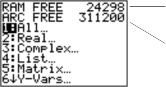
RAM FREE displays the amount of available RAM.
ARC FREE displays the amount of available Archive.
Available RAM, Archive, and App Slots
The TI-84 Plus / TI-84 Plus Silver Edition has Archive, RAM, and Application (App) slot memory for you to use and manage. The available RAM stores computations, lists, variables, and data. The available Archive lets you store programs, Apps, groups, and other variables. The App slots are actually individual sectors of Flash ROM where Apps are stored.
|
Graphing calculator |
Available RAM |
Available Archive |
App Slots |
|
TI-84 Plus |
24 Kilobytes |
491 Kilobytes |
30 |
|
TI-84 Plus Silver Edition |
24 Kilobytes |
1.5 Megabytes |
94 |
Note: Some Apps take up several App slots.
Displaying the About Screen
About displays information about the TI-84 Plus Operating System (OS) Version, Product Number, Product Identification (ID), and Flash Application (App) Certificate Revision Number. To display the About screen, press [2nd] [MEM] and then select 1:About.
Displays the type of graphing calculator.
Displays the OS version. As new software upgrades become available, you can electronically upgrade your unit.
Displays the Product ID. Each Flash-based graphing calculator has a unique product ID, which you may need if you contact technical support. You can also use this 14 digit ID to register your calculator at education.ti.com, or identify your calculator in the event that it is lost or stolen.
Displaying the MEMORY MANAGEMENT/DELETE Menu
Mem Mgmt/Del displays the MEMORY MANAGEMENT/DELETE menu. The two lines at the top report the total amount of available RAM (RAM FREE) and Archive (ARC FREE) memory. By selecting menu items on this screen, you can see the amount of memory each variable type is using. This information can help you determine if you need to delete variables from memory to make room for new data, such as programs or Apps.
To check memory usage, follow these steps.
Press [2nd] [MEM] to display the MEMORY menu.
Note: The up arrow and down arrow in the top or bottom of the left column indicate that you can scroll up or down to view more variable types.
Select 2:Mem Mgmt/Del to display the MEMORY MANAGEMENT/DELETE menu. The TI-84 Plus expresses memory quantities in bytes.
Select variable types from the list to display memory usage.
Notes: Real, List, Y-Vars, and Prgm variable types never reset to zero, even after memory is cleared.
Apps are independent applications which are stored in Flash ROM. AppVars is a variable holder used to store variables created by Apps. You cannot edit or change variables in AppVars unless you do so through the application which created them.
To leave the MEMORY MANAGEMENT/DELETE menu, press either [2nd] [QUIT] or [CLEAR]. Both options display the home screen.
Deleting an Item
To increase available memory by deleting the contents of any variable (real or complex number, list, matrix, Y= variable, program, Apps, AppVars, picture, graph database, or string), follow these steps.
Press [2nd] [MEM] to display the MEMORY menu.
Select 2:Mem Mgmt/Del to display the MEMORY MANAGEMENT/DELETE menu.
Select the type of data you want to delete, or select 1:All for a list of all variables of all types. A screen is displayed listing each variable of the type you selected and the number of bytes each variable is using.
For example, if you select 4:List, the LIST editor screen is displayed.
Press [up key] and [down key] to move the selection cursor (right facing triangle) next to the item you want to delete, and then press [DEL]. The variable is deleted from memory. You can delete individual variables one by one from this screen. No warning will be given to verify the deletion.
Note: If you are deleting programs or Apps, you will receive a message asking you to confirm this delete action. Select 2:Yes to continue.
To leave any variable screen without deleting anything, press [2nd] [QUIT], which displays the home screen.
You cannot delete some system variables, such as the last-answer variable Ans and the statistical variable RegEQ.
Clear Entries
Clear Entries clears the contents of the ENTRY (last entry on home screen) storage area. To clear the ENTRY storage area, follow these steps.
Press [2nd] [MEM] to display the MEMORY menu.
Select 3:Clear Entries to paste the instruction to the home screen.
Press [ENTER] to clear the ENTRY storage area.
![]()
To cancel Clear Entries, press [CLEAR].
Note: If you select 3:Clear Entries from within a program, the Clear Entries instruction is pasted to the program editor, and the Entry (last entry) is cleared when the program is executed.
ClrAllLists
ClrAllLists sets the dimension of each list in RAM to 0. To clear all elements from all lists, follow these steps.
Press [2nd] [MEM] to display the MEMORY menu.
Select 4:ClrAllLists to paste the instruction to the home screen.
Press [ENTER] to set the dimension of each list in memory to 0.
![]()
To cancel ClrAllLists, press [CLEAR].
ClrAllLists does not delete list names from memory, from the LIST NAMES menu, or from the stat list editor.
Note: If you select 4:ClrAllLists from within a program, the ClrAllLists instruction is pasted to the program editor. The lists are cleared when the program is executed.
Archiving and UnArchiving Variables
Archiving lets you store data, programs, or other variables to the user data archive (ARC) where they cannot be edited or deleted inadvertently. Archiving also allows you to free up RAM for variables that may require additional memory.
Archived variables cannot be edited or executed. They can only be seen and unarchived. For example, if you archive list L1, you will see that L1 exists in memory but if you select it and paste the name L1 to the home screen, you won’t be able to see its contents or edit it.
Note: Not all variables may be archived. Not all archived variables may be unarchived. For example, system variables including r, t, x, y, and theta cannot be archived. Apps and Groups always exist in Flash ROM so there is no need to archive them. Groups cannot be unarchived. However, you can ungroup or delete them.
|
Variable Type |
Names |
Archive? (yes/no) |
UnArchive? (yes/no) |
|
Real numbers |
A, B, ... , Z |
yes |
yes |
|
Complex numbers |
A, B, ... , Z |
yes |
yes |
|
Matrices |
[A], [B], [C], ... , [J] |
yes |
yes |
|
Variable Type |
Names |
Archive? (yes/no) |
UnArchive? (yes/no) |
|
Lists |
L1, L2, L3, L4, L5, L6, and user-defined names |
yes |
yes |
|
Programs |
yes |
yes |
|
|
Functions |
Y1, Y2, . . . , Y9, Y0 |
no |
not applicable |
|
Parametric equations |
X1T and Y1T, ... , X6T and Y6T |
no |
not applicable |
|
Polar functions |
r1, r2, r3, r4, r5, r6 |
no |
not applicable |
|
Sequence functions |
u, v, w |
no |
not applicable |
|
Stat plots |
Plot1, Plot2, Plot3 |
no |
not applicable |
|
Graph databases |
GDB1, GDB2,... |
yes |
yes |
|
Graph pictures |
Pic1, Pic2, ... , Pic9, Pic0 |
yes |
yes |
|
Strings |
Str1, Str2, . . . Str9, Str0 |
yes |
yes |
|
Tables |
TblStart, DeltaTbl, TblInput |
no |
not applicable |
|
Apps |
Applications |
see Note above |
no |
|
AppVars |
Application variables |
yes |
yes |
|
Groups |
see Note above |
no |
|
|
Variables with reserved names |
minX, maxX, RegEQ, and others |
no |
not applicable |
|
System variables |
Xmin, Xmax, and others |
no |
not applicable |
Archiving and unarchiving can be done in two ways:
Use the 5:Archive or 6:UnArchive commands from the MEMORY menu or CATALOG.
Use a Memory Management editor screen.
Before archiving or unarchiving variables, particularly those with a large byte size (such as large programs) use the MEMORY menu to:
Find the size of the variable.
See if there is enough free space.
|
For: |
Sizes must be such that: |
|
Archive |
Archive free size greater than variable size |
|
For: |
Sizes must be such that: |
|
UnArchive |
RAM free size greater than variable size |
Note: If there is not enough space, unarchive or delete variables as necessary. Be aware that when you unarchive a variable, not all the memory associated with that variable in user data archive will be released since the system keeps track of where the variable has been and where it is now in RAM.
Even if there appears to be enough free space, you may see a Garbage Collection message when you attempt to archive a variable. Depending on the usability of empty blocks in the user data archive, you may need to unarchive existing variables to create more free space.
To archive or unarchive a list variable (L1) using the Archive/UnArchive options from the MEMORY
menu:
Press [2nd] [MEM] to display the MEMORY menu.
Select 5:Archive or 6:UnArchive to place the command in the Home screen.
Press [2nd] [L1] to place the L1 variable in the Home screen.
![]()
Press [ENTER] to complete the archive process.
![]()
Note: An asterisk will be displayed to the left of the Archived variable name to indicate it is archived.
To archive or unarchive a list variable (L1) using a Memory Management editor:
Press [2nd] [MEM] to display the MEMORY menu.
Select 2:Mem Mgmt/Del to display the MEMORY MANAGEMENT/DELETE menu.
Select 4:List to display the LIST menu.
Press [ENTER] to archive L1. An asterisk will appear to the left of L1 to indicate it is an archived variable. To unarchive a variable in this screen, put the cursor next to the archived variable and press [ENTER]. The asterisk will disappear.
Press [2nd] [QUIT] to leave the LIST menu.
Note: You can access an archived variable for the purpose of linking, deleting, or unarchiving it, but you cannot edit it.
RAM ARCHIVE ALL Menu
Reset displays the RAM ARCHIVE ALL menu. This menu gives you the option of resetting all memory (including default settings) or resetting selected portions of memory while preserving other data stored in memory, such as programs and Y= functions. For instance, you can choose to reset all of RAM or just restore the default settings. Be aware that if you choose to reset RAM, all data and programs in RAM will be erased. For archive memory, you can reset variables (Vars), applications (Apps), or both of these. Be aware that if you choose to reset Vars, all data and programs in archive memory will be erased. If you choose to reset Apps, all applications in archive memory will be erased.
When you reset defaults on the TI-84 Plus, all defaults in RAM are restored to the factory settings. Stored data and programs are not changed.
These are some examples of TI-84 Plus defaults that are restored by resetting the defaults.
Mode settings such as Normal (notation); Func (graphing); Real (numbers); and Full (screen)
Y= functions off
Window variable values such as Xmin=-10, Xmax=10, Xscl=1, Yscl=1, and Xres=1
STAT PLOTS off
Format settings such as CoordOn (graphing coordinates on); AxesOn; and ExprOn (expression on)
rand seed value to 0
Displaying the RAM ARCHIVE ALL Menu
To display the RAM ARCHIVE ALL menu on the TI-84 Plus, follow these steps.
Press [2nd] [MEM] to display the MEMORY menu.
Select 7:Reset to display the RAM ARCHIVE ALL menu.
![]()
Resetting RAM Memory
Resetting all RAM restores RAM system variables to factory settings and deletes all nonsystem variables and all programs. Resetting RAM defaults restores all system variables to default settings without deleting variables and programs in RAM. Resetting all RAM or resetting defaults does not affect variables and applications in user data archive.
Note: Before you reset all RAM memory, consider restoring sufficient available memory by deleting only selected data.
To reset all RAM memory or RAM defaults on the TI-84 Plus, follow these steps.
From the RAM ARCHIVE ALL menu, select 1:All RAM to display the RESET RAM menu or
2:Defaults to display the RESET DEFAULTS menu.
If you are resetting RAM, read the message below the RESET RAM menu.
To cancel the reset and return to the HOME screen, press [ENTER].
To erase RAM memory or reset defaults, select 2:Reset. Depending on your choice, the message RAM cleared or Defaults set is displayed on the home screen.
Resetting Archive Memory
When resetting archive memory on the TI-84 Plus, you can choose to delete from user data archive all variables, all applications, or both variables and applications.
To reset all or part of user data archive memory, follow these steps.
From the RAM ARCHIVE ALL menu, press [right key] to display the ARCHIVE menu.
Select one of the following:
1:Vars to display the RESET ARC VARS menu.
2:Apps to display the RESET ARC APPS menu.
3:Both to display the RESET ARC BOTH menu.
Read the message below the menu.
To cancel the reset and return to the HOME screen, press [ENTER].
To continue with the reset, select 2:Reset. A message indicating the type of archive memory cleared will be displayed on the HOME screen.
Resetting All Memory
When resetting all memory on the TI-84 Plus, RAM and user data archive memory is restored to factory settings. All nonsystem variables, applications, and programs are deleted. All system variables are reset to default settings.
Before you reset all memory, consider restoring sufficient available memory by deleting only selected data.
To reset all memory on the TI-84 Plus, follow these steps.
From the RAM ARCHIVE ALL menu, press [right key] [right key] to display the ALL menu.
![]()
Select 1:All Memory to display the RESET MEMORY menu.
Read the message below the RESET MEMORY menu.
To cancel the reset and return to the HOME screen, press [ENTER].
To continue with the reset, select 2:Reset. The message MEM cleared is displayed on the
HOME screen.
When you clear memory, the contrast sometimes changes. If the screen is faded or blank, adjust the contrast by pressing [2nd] [up key] or [down key].
Grouping Variables
Grouping allows you to make a copy of two or more variables residing in RAM and then store them as a group in user data archive. The variables in RAM are not erased. The variables must exist in RAM before they can be grouped. In other words, archived data cannot be included in a group. Once grouped, the variables can be deleted from RAM to open memory. When the variables are needed later, they can be ungrouped for use.
To create a group of variables:
Press [2nd] [MEM] to display the MEMORY menu.

Select 8:Group to display GROUP UNGROUP menu.
![]()
Press [ENTER] to display the GROUP menu.
![]()
Enter a name for the new group and press [ENTER].
Note: A group name can be one to eight characters long. The first character must be a letter from A to Z or theta. The second through eighth characters can be letters, numbers, or theta.
![]()
Select the type of data you want to group. You can select 1:All+ which shows all variables of all types available and selected. You can also select 2:All- which shows all variables of all types available but not selected. A screen is displayed listing each variable of the type you selected.
For example, suppose some variables have been created in RAM, and selecting 2:All-
displays the following screen.
Press [up key] and [down key] to move the selection cursor (right facing triangle) next to the first item you want to copy into a group, and then press [ENTER]. A small square will remain to the left of all variables selected for grouping.
Repeat the selection process until all variables for the new group are selected and then press
[right key] to display the DONE menu.
![]()
Press [ENTER] to complete the grouping process.
Note: You can only group variables in RAM. You cannot group some system variables, such as the last-answer variable Ans and the statistical variable RegEQ.
Ungrouping Variables
Ungrouping allows you to make a copy of variables in a group stored in user data archive and place them ungrouped in RAM.
DuplicateName Menu
During the ungrouping action, if a duplicate variable name is detected in RAM, the DUPLICATE NAME menu is displayed.
![]()
DuplicateName
1: Rename Prompts to rename receiving variable.
2: Overwrite Overwrites data in receiving duplicate variable.
3: Overwrite All Overwrites data in all receiving duplicate
variables.
4: Omit Skips ungrouping of sending variable.
5: Quit Stops ungrouping at duplicate variable.
![]()
Notes about Menu Items:
When you select 1:Rename, the Name= prompt is displayed, and alpha-lock is on. Enter a new variable name, and then press [ENTER]. Ungrouping resumes.
When you select 2:Overwrite, the unit overwrites the data of the duplicate variable name found in RAM. Ungrouping resumes.
When you select 3: Overwrite All, the unit overwrites the data of all duplicate variable names found in RAM. Ungrouping resumes.
When you select 4:Omit, the unit does not ungroup the variable in conflict with the duplicated variable name found in RAM. Ungrouping resumes with the next item.
When you select 5:Quit, ungrouping stops, and no further changes are made. To ungroup a group of variables:
Press [2nd] [MEM] to display the MEMORY menu.
Select 8:Group to display the GROUP UNGROUP menu.
Press [right key] to display the UNGROUP menu.
Press [up key] and [down key] to move the selection cursor (right facing triangle) next to the group variable you want to ungroup, and then press [ENTER].
The ungroup action is completed.
Note: Ungrouping does not remove the group from user data archive. You must delete the group in user data archive to remove it.
Garbage Collection Message
If you use the user data archive extensively, you may see a Garbage Collect? message. This occurs if you try to archive a variable when there is not enough free contiguous archive memory.
The Garbage Collect? message lets you know an archive will take longer than usual. It also alerts you that the archive will fail if there is not enough memory.
The message can also alert you when a program is caught in a loop that repetitively fills the user data archive. Select No to cancel the garbage collection process, and then find and correct the errors in your program.
When YES is selected, the TI-84 Plus will attempt to rearrange the archived variables to make additional room.
Responding to the Garbage Collection Message
To cancel, select 1:No.
If you select 1:No, the message
ERR:ARCHIVE FULL will be displayed.
To continue archiving, select 2:Yes.
If you select 2:Yes, the process message Garbage Collecting... or Defragmenting... will be displayed.
Note: The process message Defragmenting... is displayed whenever an application marked for deletion is encountered. Garbage collection may take up to 20 minutes, depending on how much of archive memory has been used to store variables.
After garbage collection, depending on how much additional space is freed, the variable may or may not be archived. If not, you can unarchive some variables and try again.
Why Is Garbage Collection Necessary?
The user data archive is divided into sectors. When you first begin archiving, variables are stored consecutively in sector 1. This continues to the end of the sector.
An archived variable is stored in a continuous block within a single sector. Unlike an application stored in user data archive, an archived variable cannot cross a sector boundary. If there is not enough space left in the sector, the next variable is stored at the beginning of the next sector. Typically, this leaves an empty block at the end of the previous sector.
variable A
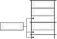
Sector 1
variable B
Empty block
variable D
variable C
Sector 2
Depending on its size, variable D is stored in one of these locations.
Sector 3
Each variable that you archive is stored in the first empty block large enough to hold it.
This process continues to the end of the last sector. Depending on the size of individual variables, the empty blocks may account for a significant amount of space. Garbage collection occurs when the variable you are archiving is larger than any empty block.
How Unarchiving a Variable Affects the Process
When you unarchive a variable, it is copied to RAM but it is not actually deleted from user data archive memory. Unarchived variables are “marked for deletion,†meaning they will be deleted during the next garbage collection.
After you unarchive variables B and C, they continue to take up space.
variable A
Sector 1
Sector 2
variable D
Sector 3
If the MEMORY Screen Shows Enough Free Space
Even if the MEMORY screen shows enough free space to archive a variable or store an application, you may still get a Garbage Collect? message or an ERR: ARCHIVE FULL message.
When you unarchive a variable, the Archive free amount increases immediately, but the space is not actually available until after the next garbage collection.
If the Archive free amount shows enough available space for your variable, there probably will be enough space to archive it after garbage collection (depending on the usability of any empty blocks).
The Garbage Collection Process
The garbage collection process:
Deletes unarchived variables from the user data archive.
Rearranges the remaining variables into consecutive blocks.
variable A variable D

Sector 1
Sector 2
Note: Power loss during garbage collection may cause all memory (RAM and Archive) to be deleted.
Using the GarbageCollect Command
You can reduce the number of automatic garbage collections by periodically optimizing memory. This is done by using the GarbageCollect command.
To use the GarbageCollect command, follow these steps.
From the HOME screen, press [2nd] [CATALOG] to display the CATALOG.
Press [down key] or [up key] to scroll the CATALOG until the selection cursor points to the
GarbageCollect command or press G to skip to the commands starting with the letter G.
Press [ENTER] to paste the command to the HOME screen.
Press [ENTER] to display the Garbage Collect? message.
Select 2:Yes to begin garbage collection.
Even if the MEMORY screen shows enough free space to archive a variable or store an application, you may still get an ERR: ARCHIVE FULL message.
An ERR:ARCHIVE FULL message may be displayed:
When there is insufficient space to archive a variable within a continuous block and within a single sector.
When there is insufficient space to store an application within a continuous block of memory.
When the message is displayed, it will indicate the largest single space of memory available for storing a variable and an application.
To resolve the problem, use the GarbageCollect command to optimize memory. If memory is still insufficient, you must delete variables or applications to increase space.
Getting Started is a fast-paced introduction. Read the chapter for details.
Create and store a variable and a matrix, and then transfer them to another TI-84 Plus.
On the home screen of the sending unit, press 5 [.] 5 [STO right arrow] [ALPHA] Q. Press [ENTER] to store 5.5 to Q.
Press [ALPHA] [F3] [down key] [down key] [ENTER] to display the 2x2 matrix template. Press 1 [right key] 2 [right key] 3 [right key] 4 [right key] to enter the values. Press [STO right arrow] [2nd] [MATRIX] 1 [ENTER] to store the matrix to [A].

On the sending unit, press [2nd] [MEM]
to display the MEMORY menu.

On the sending unit, press 2 to select 2:Mem Mgmt/Del. The MEMORY MANAGEMENT menu is displayed.
![]()
On the sending unit, press 5 to select 5:Matrix. The MATRIX editor screen is displayed.
![]()
On the sending unit, press [ENTER] to archive [A]. An asterisk (*) will appear, signifying that [A] is now archived.
Connect the graphing calculators with the USB unit-to-unit cable. Push both ends in firmly.
![]()
On the receiving unit, press [2nd] [LINK] [right key] to display the RECEIVE menu. Press 1 to select 1:Receive. The message Waiting... is displayed and the busy indicator is on.
On the sending unit, press [2nd] [LINK]
to display the SEND menu.
Press 2 to select 2:All-. The All- SELECT
screen is displayed.
Press [down key] until the selection cursor ( â–º ) is next to [A] MATRX. Press [ENTER].
Press [down key] until the selection cursor is next to Q REAL. Press [ENTER]. A square dot next to [A] and Q indicates that each is selected to send.
![]()
On the sending unit, press [right key] to display the TRANSMIT menu.
On the sending unit, press 1 to select 1:Transmit and begin transmission. The receiving unit displays the message Receiving....When the items are transmitted, both units display the name and type of each transmitted variable.
This chapter describes how to communicate with compatible TI units. The TI-84 Plus has a USB port to connect and communicate with another TI-84 series calculator. A USB unit-to-unit cable is included with the TI-84 Plus.
The TI-84 Plus also has an I/O port using a I/O unit-to-unit cable to communicate with:
TI-83 Plus Silver Edition
TI-83 Plus
TI-83
TI-82
TI-73
CBL 2â„¢ or a CBRâ„¢
You can send items from a calculator with an older OS to a calculator with OS 2.53MP and higher. However, you may receive a version error if you send items from a calculator with OS 2.53MP or higher to a calculator with an older OS. Transferring files between calculators works best if both calculators have the latest operating system software installed. For example, if you send a list that contains fractions (OS 2.53MP and higher) to a calculator with OS 2.43, a version error displays because OS 2.43 does not support fractions.
Connecting Two Graphing Calculators with a USB Unit-to-Unit Cable or an I/O Unit-to-Unit Cable
USB Unit-to-Unit Cable
The TI-84 Plus USB link port is located at the top right edge of the graphing calculator.
Firmly insert either end of the USB unit-to-unit cable into the USB port.
Insert the other end of the cable into the other graphing calculator’s USB port.
I/O Unit-to-Unit Cable
The TI-84 Plus I/O link port is located at the top left edge of the graphing calculator.
Firmly insert either end of the I/O unit-to-unit cable into the port.
Insert the other end of the cable into the other graphing calculator’s I/O port.
TI-84 Plus to a TI-83 Plus using I/O Unit-to-Unit Cable
The TI-84 Plus I/O link port is located at the top left edge of the graphing calculator. The TI-83 Plus I/O link port is located at the bottom edge of the graphing calculator.
Firmly insert either end of the I/O unit-to-unit cable into the port.
Insert the other end of the cable into the other graphing calculator’s I/O port.
Linking to the CBL/CBR System
The CBL 2â„¢ system and the CBRâ„¢ system are optional accessories that also connect to a TI-84 Plus with the I/O unit-to-unit cable. With a CBL 2â„¢ system or CBRâ„¢ system and a TI-84 Plus, you can collect and analyze real-world data.
Linking to a Computer
With TI Connectâ„¢ software and the USB computer cable that is included with your TI-84 Plus, you can link the graphing calculator to a personal computer.
LINK SEND Menu
To display the LINK SEND menu, press [2nd] [LINK].
![]()
SEND RECEIVE
|
1: |
All+... |
Displays all items as selected, including RAM and Flash applications. |
|
2: |
All-... |
Displays all items as deselected. |
|
3: |
Prgm... |
Displays all program names. |
|
4: |
List... |
Displays all list names. |
|
5: |
Lists to |
Displays list names L1 through L6. |
|
TI82... |
||
|
6: |
GDB... |
Displays all graph databases. |
|
7: |
Pic... |
Displays all picture data types. |
|
8: |
Matrix... |
Displays all matrix data types. |
|
9: |
Real... |
Displays all real variables. |
|
0: |
Complex... |
Displays all complex variables. |
|
A: |
Y-Vars... |
Displays all Y= variables. |
|
B: |
String... |
Displays all string variables. |
|
C: |
Apps... |
Displays all software applications. |
|
D: |
AppVars... |
Displays all software application variables. |
|
E: |
Group... |
Displays all grouped variables. |
|
F: |
SendId |
Sends the Calculator ID number immediately. (You do not need to select SEND.) |
|
G: |
SendOS |
Sends operating system updates to another TI-84 Plus Silver Edition or TI-84 Plus. You can |
|
not send the operating system to the TI-83 Plus |
||
|
product family. |
||
|
H: |
Back Up... |
Selects all RAM and mode settings (no Flash applications or archived items) for backup to |
|
another TI-84 Plus, TI-84 Plus Silver Edition, |
||
|
TI-83 Plus Silver Edition, or to a TI-83 Plus. |
When you select an item on the LINK SEND menu, the corresponding SELECT screen is displayed.
Note: Each SELECT screen, except All+…, is initially displayed with nothing pre-selected. All+… is displayed with everything pre-selected.
To select items to send:
Press [2nd] [LINK] on the sending unit to display the LINK SEND menu.
Select the menu item that describes the data type to send. The corresponding SELECT screen is displayed.
Press [up key] and [down key] to move the selection cursor ( â–º ) to an item you want to select or deselect.
Press [ENTER] to select or deselect the item. Selected names are marked with a solid rectangle.
Note: An asterisk (*) to the left of an item indicates the item is archived.
Repeat steps 3 and 4 to select or deselect additional items.
Sending the Selected Items
After you have selected items to send on the sending unit and set the receiving unit to receive, follow these steps to transmit the items. To set the receiving unit, see Receiving Items.
Press [right key] on the sending unit to display the TRANSMIT menu.
![]()
Confirm that Waiting... is displayed on the receiving unit, which indicates it is set to receive.
Press [ENTER] to select 1:Transmit. The name and type of each item are displayed line-by-line on the sending unit as the item is queued for transmission, and then on the receiving unit as each item is accepted.
Note: Items sent from the RAM of the sending unit are transmitted to the RAM of the receiving unit. Items sent from user data archive (flash) of the sending unit are transmitted to user data archive (flash) of the receiving unit.
After all selected items have been transmitted, the message Done is displayed on both calculators. Press [up key] and [down key] to scroll through the names.
Sending to a TI-84 Plus Silver Edition or TI-84 Plus
You can transfer variables (all types), programs, and Flash applications to another TI-84 Plus Silver Edition or TI-84 Plus. You can also backup the RAM memory of one unit to another.
Note: Keep in mind that the TI-84 Plus has less Flash memory than the TI-84 Plus Silver Edition.
Variables stored in RAM on the sending TI-84 Plus Silver Edition will be sent to the RAM of the receiving TI-84 Plus Silver Edition or TI-84 Plus.
Variables and applications stored in the user data archive of the sending TI-84 Plus Silver Edition will be sent to the user data archive of the receiving TI-84 Plus Silver Edition or TI-84 Plus.
After sending or receiving data, you can repeat the same transmission to additional TI-84 Plus Silver Edition or TI-84 Plus units—from either the sending unit or the receiving unit—without having to reselect data to send. The current items remain selected. However, you cannot repeat transmission if you selected All+ or All-.
To send data to an additional TI-84 Plus Silver Edition or a TI-84 Plus:
Use a USB unit-to-unit cable to link two units together.
On the sending unit press [2nd] [LINK] and select a data type and items to SEND.
Press [right key] on the sending unit to display the TRANSMIT menu.
On the other unit, press [2nd] [LINK] [right key] to display the RECEIVE menu.
Press [ENTER] on the receiving unit.
Press [ENTER] on the sending unit. A copy of the selected item(s) is sent to the receiving unit.
Disconnect the link cable only from the receiving unit and connect it to another unit.
Press [2nd] [LINK] on the sending unit.
Select only the data type. For example, if the unit just sent a list, select 4:LIST.
Note: The item(s) you want to send are pre-selected from the last transmission. Do not select or deselect any items. If you select or deselect an item, all selections or deselections from the last transmission are cleared.
Press [right key] on the sending unit to display the TRANSMIT menu.
On the new receiving unit, press [2nd] [LINK] [right key] to display the RECEIVE menu.
Press [ENTER] on the receiving unit.
Press [ENTER] on the sending unit. A copy of the selected item(s) is sent to the receiving unit.
Repeat steps 7 through 13 until the items are sent to all additional units.
Sending to a TI-83 Plus or TI-83 Plus Silver Edition
You can send all variables from a TI-84 Plus to a TI-83 Plus or TI-83 Plus Silver Edition except
Flash applications with new features, or programs with new features in them.
If archived variables on the TI-84 Plus are variable types recognized and used on the TI-83 Plus or TI-83 Plus Silver Edition, you can send these variables to the TI-83 Plus or TI-83 Plus Silver Edition. They will be automatically sent to the RAM of the TI-83 Plus or TI-83 Plus Silver Edition during the transfer process. It will send to archive if the item is from archive.
To send data to a TI-83 Plus or TI-83 Plus Silver Edition:
Use an I/O unit-to-unit cable to link the two units together.
Set the TI-83 Plus or TI-83 Plus Silver Edition to receive.
Press [2nd] [LINK] on the sending TI-84 Plus to display the LINK SEND menu.
Select the menu of the items you want to transmit.
Press [right key] on the sending TI-84 Plus to display the LINK TRANSMIT menu.
Confirm that the receiving unit is set to receive.
Press [ENTER] on the sending TI-84 Plus to select 1:Transmit and begin transmitting.
LINK RECEIVE Menu
To display the LINK RECEIVE menu, press [2nd] [LINK] [right key].
![]()
SEND RECEIVE
1: Receive Sets unit to receive data transmission.
![]()
Receiving Unit
When you select 1:Receive from the LINK RECEIVE menu on the receiving unit, the message Waiting... and the busy indicator are displayed. The receiving unit is ready to receive transmitted items. To exit the receive mode without receiving items, press [ON], and then select 1:Quit from the Error in Xmit menu.
When transmission is complete, the unit exits the receive mode. You can select 1:Receive again to receive more items. The receiving unit then displays a list of items received. Press [2nd] [QUIT] to exit the receive mode.
DuplicateName Menu
During transmission, if a variable name is duplicated, the DuplicateName menu is displayed on the receiving unit.
![]()
DuplicateName
![]()
1: Rename Prompts to rename receiving variable. 2: Overwrite Overwrites data in receiving variable. 3: Omit Skips transmission of sending variable. 4: Quit Stops transmission at duplicate variable.
When you select 1:Rename, the Name= prompt is displayed, and alpha-lock is on. Enter a new variable name, and then press [ENTER]. Transmission resumes.
When you select 2:Overwrite, the sending unit’s data overwrites the existing data stored on the receiving unit. Transmission resumes.
When you select 3:Omit, the sending unit does not send the data in the duplicated variable name. Transmission resumes with the next item.
When you select 4:Quit, transmission stops, and the receiving unit exits receive mode.
Receiving from a TI-84 Plus Silver Edition or TI-84 Plus
The TI-84 Plus Silver Edition and the TI-84 Plus are totally compatible. Keep in mind, however that the TI-84 Plus has less Flash memory than a TI-84 Plus Silver Edition.
You cannot send memory backups between the TI-84 Plus product family and the TI-83 Plus product family.
Receiving from a TI-83 Plus Silver Edition or TI-83 Plus
The TI-84 Plus product family and the TI-83 Plus product family are compatible with a few exceptions.
Receiving from a TI-83
You can transfer all variables and programs from a TI-83 to a TI-84 Plus if they fit in the RAM of the TI-84 Plus. The RAM of the TI-84 Plus is slightly less than the RAM of the TI-83.
Warning: H:Back Up overwrites the RAM memory and mode settings in the receiving unit. All information in the RAM memory of the receiving unit is lost.
Note: Archived items on the receiving unit are not overwritten.
You can backup the contents of RAM memory and mode settings (no Flash applications or archived items) to another TI-84 Plus Silver Edition. You can also backup RAM memory and mode settings to a TI-84 Plus. The backup calculator must also have OS 2.55MP installed.
To perform a RAM memory backup:
Use a USB unit-to-unit cable to link two TI-84 Plus units, or a TI-84 Plus and a TI-84 Plus Silver Edition together.
On the sending unit press [2nd] [LINK] and select H:Back Up. The MEMORYBACKUP screen displays.
![]()
On the receiving unit, press [2nd] [LINK] [right key] to display the RECEIVE menu.
Press [ENTER] on the receiving unit.
Press [ENTER] on the sending unit. A WARNING — Backup message displays on the receiving unit.
Press [ENTER] on the receiving unit to continue the backup.
— or —
Press 2:Quit on the receiving unit to cancel the backup and return to the LINK SEND menu
Note: If a transmission error is returned during a backup, the receiving unit is reset.
Memory Backup Complete
When the backup is complete, both the sending graphing calculator and receiving graphing calculator display a confirmation screen.
![]()
A transmission error occurs after one or two seconds if:
A cable is not attached to the sending unit.
A cable is not attached to the receiving unit.
Note: If the cable is attached, push it in firmly and try again.
The receiving unit is not set to receive transmission.
You attempt a backup between a TI-73, TI-82, TI-83, TI-83 Plus, or TI-83 Plus Silver Edition.
You attempt a data transfer from a TI-84 Plus to a TI-83 Plus, TI-83 Plus Silver Edition, TI-83, TI-82, or TI-73 with variables or features not recognized by the TI-83 Plus, TI-83 Plus Silver Edition, TI-83, TI-82, or TI-73.
New variable types and features not recognized by the TI-83, TI-83 Plus, TI-82, or TI-73 include applications, application variables, grouped variables, new variable types, or programs with new features in them such as Archive, UnArchive, SendID, SendOS, Asm(, AsmComp(, AsmPrgm, checkTmr(, ClockOff, ClockOn, dayOfWk(, getDate, getDtFmt, getDtStr(, getTime, getTmFmt, getTmStr, isClockOn, randIntNoRep(, setDate(, setDtFmt(, setTime(, setTmFmt(, startTmr, summation(, timeCnv and fractions.
You attempt a data transfer from a TI-84 Plus to a TI-82 with data other than real lists L1
through L6 or without using menu item 5:Lists to TI82.
You attempt a data transfer from a TI-84 Plus to a TI-73 with data other than real numbers, pics, real lists L1 through L6 or named lists with theta as part of the name.
Although a transmission error does not occur, these two conditions may prevent successful transmission.
You try to use Get( with a graphing calculator instead of a CBL 2â„¢ system or CBRâ„¢ system.
You try to use GetCalc( with a TI-83 instead of a TI-84 Plus or TI-84 Plus Silver Edition.
Insufficient Memory in Receiving Unit
During transmission, if the receiving unit does not have sufficient memory to receive an item, the Memory Full menu is displayed on the receiving unit.
To skip this item for the current transmission, select 1:Omit. Transmission resumes with the next item.
To cancel the transmission and exit receive mode, select 2:Quit.
Functions return a value, list, or matrix. You can use functions in an expression. Instructions initiate an action. Some functions and instructions have arguments. Optional arguments and accompanying commas are enclosed in brackets ( [ ] ). For details about an item, including argument descriptions and restrictions, turn to the page listed on the right side of the table.
From the CATALOG, you can paste any function or instruction to the home screen or to a command line in the program editor. However, some functions and instructions are not valid on the home screen. The items in this table appear in the same order as they appear in the CATALOG.
A dagger indicates either keystrokes that are valid in the program editor only or ones that paste certain instructions when you are in the program editor. Some keystrokes display menus that are available only in the program editor. Others paste mode, format, or table-set instructions only when you are in the program editor.
![]()
Function or Instruction/Arguments Result
![]()
abs(value) Returns the absolute value of a real number, expression, list, or matrix.
Key or Keys/Menu or Screen/Item
[MATH]
NUM
1:abs(
![]()
abs(complex value) Returns the magnitude of a complex number or list. [MATH]
CPX
![]()
5:abs(
valueA and valueB Returns 1 if both valueA and valueB are not equal to 0.
valueA and valueB can be real numbers, expressions, or lists.
![]()
angle(value) Returns the polar angle of a complex number or list of
complex numbers.
[2nd] [TEST]
LOGIC
1:and
[MATH]
CPX
![]()
4:angle(
ANOVA(list1,list2
[,list3,...,list20])
Performs a one-way analysis of variance for comparing the means of two to 20 populations.
[STAT] TESTS H:ANOVA(
![]()
![]()
Ans Returns the last answer. [2nd] [ANS]
Archive Moves the specified variables from RAM to the user data archive memory.
[2nd] [MEM]
5:Archive
![]()
Asm(assemblyprgmname) Executes an assembly language program. [2nd] [CATALOG]
![]()
Asm(
![]()
AsmComp(prgmASM1, prgmASM2)
Compiles an assembly language program written in ASCII and stores the hex version.
[2nd] [CATALOG]
AsmComp(
![]()
AsmPrgm Must be used as the first line of an assembly language program.
[2nd] [CATALOG]
AsmPrgm
augment(matrixA,
matrixB)
Returns a matrix, which is matrixB appended to matrixA as new columns.
[2nd] [MATRIX]
MATH
7:augment(
![]()
![]()
Function or Instruction/Arguments Result
![]()
augment(listA,listB) Returns a list, which is listB concatenated to the end of
listA.
Key or Keys/Menu or Screen/Item
[2nd] [LIST]
OPS
9:augment(
![]()
AUTO Answer Displays answers in a similar format as the input. [MODE]
Answers: AUTO
![]()
AxesOff Turns off the graph axes. dagger [2nd] [FORMAT]
AxesOff
![]()
AxesOn Turns on the graph axes. dagger [2nd] [FORMAT]
![]()
AxesOn
a+bi Sets the mode to rectangular complex number mode (a+bi).
![]()
bal(npmt[,roundvalue]) Computes the balance at npmt for an amortization
![]()
schedule using stored values for PV, I%, and PMT and rounds the computation to roundvalue.
dagger [MODE]
a+bi
[APPS] 1:Finance CALC
9:bal(
binomcdf(numtrials,p
[,x])
![]()
binompdf(numtrials,p
[,x])
Computes a cumulative probability at x for the discrete binomial distribution with the specified numtrials and probability p of success on each trial.
![]()
Computes a probability at x for the discrete binomial distribution with the specified numtrials and probability p of success on each trial.
[2nd] [DISTR]
DISTR
B:binomcdf(
[2nd] [DISTR]
DISTR
A:binompdf(
checkTmr(starttime) Returns the number of seconds since you used startTmr
to start the timer. The starttime is the value displayed by
![]()
startTmr.
[2nd] [CATALOG]
checkTmr(
chi square cdf(lowerbound, upperbound,df)
![]()
Computes the chi square distribution probability between lowerbound and upperbound for the specified degrees of freedom df.
[2nd] [DISTR]
DISTR
8:chi square cdf(
chi square pdf(x,df) Computes the probability density function (pdf) for the chi
![]()
square distribution at a specified x value for the specified degrees of freedom df.
[2nd] [DISTR]
DISTR
7:chi square pdf(
chi square- Test(observedmatrix, expectedmatrix [,drawflag])
![]()
chi square
GOF-Test(observedlist,exp ectedlist,df)
Performs a chi-square test. drawflag=1 draws results;
drawflag=0 calculates results.
Performs a test to confirm that sample data is from a population that conforms to a specified distribution.
dagger [STAT]
TESTS
C:chi square-Test(
dagger [STAT]
TESTS
D:chi square GOF- Test(
![]()
Circle(X,Y,radius) Draws a circle with center (X,Y) and radius. [2nd] [DRAW]
DRAW
![]()
9:Circle(
CLASSIC Displays inputs and outputs on a single line, such as 1/2+3/4.
[MODE]
CLASSIC
![]()
![]()
Function or Instruction/Arguments Result
Key or Keys/Menu or Screen/Item
![]()
Clear Entries Clears the contents of the Last Entry storage area. [2nd] [MEM]
MEMORY
3:Clear Entries
![]()
ClockOff Turns off the clock display in the mode screen. [2nd] [CATALOG]
ClockOff
![]()
ClockOn Turns on the clock display in the mode screen. [2nd] [CATALOG]
ClockOn
![]()
ClrAllLists Sets to 0 the dimension of all lists in memory. [2nd] [MEM]
MEMORY
4:ClrAllLists
![]()
ClrDraw Clears all drawn elements from a graph or drawing. [2nd] [DRAW]
DRAW
1:ClrDraw
![]()
![]()
ClrHome Clears the home screen. dagger [PRGM] I/O 8:ClrHome
ClrList listname1 [,listname2, ..., listname n]
Sets to 0 the dimension of one or more listnames. [STAT]
EDIT
4:ClrList
![]()
ClrTable Clears all values from the table. dagger [PRGM]
![]()
I/O 9:ClrTable
conj(value) Returns the complex conjugate of a complex number or list
of complex numbers.
![]()
Connected Sets connected plotting mode; resets all Y= editor graph-
style settings to line.
[MATH]
CPX
1:conj(
dagger [MODE]
Connected
![]()
CoordOff Turns off cursor coordinate value display. dagger [2nd]
[FORMAT]
CoordOff
![]()
CoordOn Turns on cursor coordinate value display. dagger [2nd]
[FORMAT]
![]()
![]()
CoordOn cos(value) Returns cosine of a real number, expression, or list. [COS]
cos superscript -1
![]()
(value)
Returns arccosine of a real number, expression, or list. [2nd] [COS
superscript -1]
cosh(value) Returns hyperbolic cosine of a real number, expression, or
![]()
list.
[2nd] [CATALOG]
cosh(
cosh superscript -1 (value)
![]()
CubicReg [Xlistname, Ylistname,freqlist, regequ]
Returns hyperbolic arccosine of a real number, expression, or list.
Fits a cubic regression model to Xlistname and Ylistname with frequency freqlist, and stores the regression equation to regequ.
[2nd] [CATALOG]
cosh superscript - 1(
[STAT]
CALC
6:CubicReg
![]()
![]()
Function or Instruction/Arguments Result
![]()
cumSum(list) Returns a list of the cumulative sums of the elements in
list, starting with the first element.
![]()
cumSum(matrix) Returns a matrix of the cumulative sums of matrix
![]()
elements. Each element in the returned matrix is a cumulative sum of a matrix column from top to bottom.
Key or Keys/Menu or Screen/Item
[2nd] [LIST]
OPS
6:cumSum(
[2nd] [MATRIX]
MATH
0:cumSum(
dayOfWk(year,month, day)
![]()
Returns an integer from 1 to 7, with each integer representing a day of the week. Use dayOfWk( to determine on which day of the week a particular date would occur. The year must be 4 digits; month and day can be 1 or 2 digit.
[2nd] [CATALOG]
dayOfWk( 1:Sunday 2:Monday 3:Tuesday...
dbd(date1,date2) Calculates the number of days between date1 and date2
using the actual-day-count method.
[APPS] 1:Finance CALC
D:dbd(
![]()
DEC Answers Displays answers as integers or decimal numbers. [MODE]
![]()
Answers: DEC
valueâ–ºDec Displays a real or complex number, expression, list, or matrix in decimal format.
[MATH]
MATH
2:â–ºDec
![]()
Degree Sets degree angle mode. dagger [MODE]
Degree
![]()
DelVar variable Deletes from memory the contents of variable. dagger [PRGM]
CTL
G:DelVar
![]()
DependAsk Sets table to ask for dependent-variable values. dagger [2nd]
[TBLSET]
![]()
Depend: Ask
DependAuto Sets table to generate dependent-variable values
automatically.
dagger [2nd] [TBLSET]
Depend: Auto
![]()
det(matrix) Returns determinant of matrix. [2nd] [MATRIX]
MATH
![]()
1:det(
DiagnosticOff Sets diagnostics-off mode; r, r square, and R square are
not displayed as regression model results.
![]()
DiagnosticOn Sets diagnostics-on mode; r, r square, and R square are
displayed as regression model results.
[2nd] [CATALOG]
DiagnosticOff
[2nd] [CATALOG]
DiagnosticOn
![]()
dim(listname) Returns the dimension of listname. [2nd] [LIST]
OPS
3:dim(
![]()
dim(matrixname) Returns the dimension of matrixname as a list. [2nd] [MATRIX]
MATH
3:dim(
![]()
![]()
![]()
Function or Instruction/Arguments Result
Key or Keys/Menu or Screen/Item
length right arrow
dim(listname)
Assigns a new dimension (length) to a new or existing
listname.
[2nd] [LIST]
OPS
![]()
3:dim(
{rows,columns} right arrow dim(matrixname)
Assigns new dimensions to a new or existing matrixname. [2nd] [MATRIX]
MATH
3:dim(
![]()
Disp Displays the home screen. dagger [PRGM]
![]()
I/O 3:Disp
Disp [valueA,valueB,
valueC,...,value n]
Displays each value. dagger [PRGM]
I/O 3:Disp
![]()
DispGraph Displays the graph. dagger [PRGM] I/O 4:DispGraph
![]()
DispTable Displays the table. dagger [PRGM] I/O 5:DispTable
![]()
![]()
valueâ–ºDMS Displays value in DMS format. [2nd] [ANGLE] ANGLE 4:â–ºDMS
Dot Sets dot plotting mode; resets all Y= editor graph-style settings to dot.
dagger [MODE]
Dot
![]()
DrawF expression Draws expression (in terms of X) on the graph. [2nd] [DRAW]
DRAW
![]()
6:DrawF
DrawInv expression Draws the inverse of expression by plotting X values on the
y-axis and Y values on the x-axis.
[2nd] [DRAW]
DRAW
![]()
8:DrawInv
:DS<(variable,value)
:commandA
:commands
Decrements variable by 1; skips commandA if variable <
value.
dagger [PRGM]
CTL B:DS<(
![]()
e Returns e. [2nd] [e]
![]()
e^(power) Returns e raised to power. [2nd] [e superscript x]
![]()
e^(list) Returns a list of e raised to a list of powers. [2nd] [e superscript
![]()
x]
Exponent:
valueEexponent
![]()
Exponent:
listEexponent
![]()
Exponent:
matrixEexponent
Returns value times 10 to the exponent. [2nd] [EE]
Returns list elements times 10 to the exponent. [2nd] [EE]
Returns matrix elements times 10 to the exponent. [2nd] [EE]
![]()
![]()
![]()
Function or Instruction/Arguments Result
Key or Keys/Menu or Screen/Item
â–ºEff(nominal rate, compounding periods)
![]()
Else
![]()
See If:Then:Else
Computes the effective interest rate. [APPS] 1:Finance CALC
C:â–ºEff(
End Identifies end of For(, If-Then-Else, Repeat, or While
loop.
dagger [PRGM]
CTL
7:End
![]()
Eng Sets engineering display mode. dagger [MODE]
![]()
Eng
Equâ–ºString(Y=
var,Strn)
Converts the contents of a Y= var to a string and stores it in
Strn.
[2nd] [CATALOG]
Equâ–ºString(
![]()
expr(string) Converts string to an expression and executes it. [2nd] [CATALOG]
![]()
expr(
ExpReg [Xlistname,
Ylistname,freqlist,regequ]
Fits an exponential regression model to Xlistname and Ylistname with frequency freqlist, and stores the regression equation to regequ.
[STAT]
CALC
0:ExpReg
![]()
ExprOff Turns off the expression display during TRACE. dagger [2nd]
[FORMAT]
ExprOff
![]()
ExprOn Turns on the expression display during TRACE. dagger [2nd]
[FORMAT]
![]()
ExprOn
![]()
F cdf(lowerbound, upperbound, numerator df, denominator df)
Computes the F distribution probability between lowerbound and upperbound for the specified numerator df (degrees of freedom) and denominator df.
[2nd] [DISTR]
DISTR
0:Fcdf(
â–º F â—„ â–ºD Converts an answer from a fraction to a decimal or from a
decimal to a fraction.
[ALPHA] [F1]
4: â–º F â—„ â–º D
or [MATH] NUM
8: â–º F â—„ â–º D
![]()
Fill(value,matrixname) Stores value to each element in matrixname. [2nd] [MATRIX]
MATH
4:Fill(
![]()
Fill(value,listname) Stores value to each element in listname. [2nd] [LIST]
OPS
4:Fill(
![]()
Fix # Sets fixed-decimal mode for # of decimal places. dagger [MODE]
0123456789
(select one)
![]()
Float Sets floating decimal mode. dagger [MODE]
Float
![]()
![]()
![]()
Function or Instruction/Arguments Result
Key or Keys/Menu or Screen/Item
fMax(expression, variable,lower,upper [,tolerance])
![]()
fMin(expression,variable,
lower,upper[,tolerance])
![]()
fnInt(expression,variable,
lower,upper[,tolerance])
Returns the value of variable where the local maximum of expression occurs, between lower and upper, with specified tolerance.
Returns the value of variable where the local minimum of expression occurs, between lower and upper, with specified tolerance.
Returns the function integral of expression with respect to
variable, between lower and upper, with specified tolerance.
[MATH]
MATH
7:fMax(
[MATH]
MATH
6:fMin(
[MATH]
MATH
![]()
9:fnInt(
FnOff [function#,
function#,...,function n]
![]()
FnOn [function#,
function#,...,function n]
Deselects all Y= functions or specified Y= functions. [VARS]
Y-VARS
4:On/Off 2:FnOff
Selects all Y= functions or specified Y= functions. [VARS]
Y-VARS
![]()
4:On/Off 1:FnOn
:For(variable,begin,end
[,increment])
:commands
:End
![]()
:commands
Executes commands through End, incrementing variable
from begin by increment until variable>end.
dagger [PRGM]
CTL
4:For(
fPart(value) Returns the fractional part or parts of a real or complex
number, expression, list, or matrix.
[MATH]
NUM
![]()
4:fPart(
Fpdf(x,numerator df, denominator df)
Computes the F distribution probability between lowerbound and upperbound for the specified numerator df (degrees of freedom) and denominator df.
[2nd] [DISTR]
DISTR
9:Fpdf(
![]()
FRAC Answers Displays answers as fractions, if possible. [MODE]
![]()
Answers: FRAC
valueâ–ºFrac Displays a real or complex number, expression, list, or
matrix as a fraction simplified to its simplest terms.
[MATH]
MATH
1:â–ºFrac
![]()
Full Sets full screen mode. dagger [MODE]
Full
![]()
Func Sets function graphing mode. dagger [MODE]
![]()
Func
GarbageCollect Displays the garbage collection menu to allow cleanup of
unused archive memory.
![]()
gcd(valueA,valueB) Returns the greatest common divisor of valueA and valueB,
which can be real numbers or lists.
[2nd] [CATALOG]
GarbageCollect
[MATH]
NUM
9:gcd(
![]()
![]()
Function or Instruction/Arguments Result
![]()
geometcdf(p,x) Computes a cumulative probability at x, the number of the
trial on which the first success occurs, for the discrete geometric distribution with the specified probability of success p.
![]()
geometpdf(p,x) Computes a probability at x, the number of the trial on which
the first success occurs, for the discrete geometric distribution with the specified probability of success p.
![]()
Get(variable) Gets data from the CBL 2â„¢ or CBRâ„¢ System and stores it
in variable.
Key or Keys/Menu or Screen/Item
[2nd] [DISTR]
DISTR
F:geometcdf(
[2nd] [DISTR]
DISTR
E:geometpdf(
dagger [PRGM]
![]()
I/O A:Get(
GetCalc(variable
[,portflag])
Gets contents of variable on another TI-84 Plus and stores it to variable on the receiving TI-84 Plus. By default, the TI-84 Plus uses the USB port if it is connected. If the USB cable is not connected, it uses the I/O port.
portflag=0 use USB port if connected;
portflag=1 use USB port;
![]()
portflag=2 use I/O port.
dagger [PRGM] I/O 0:GetCalc(
getDate Returns a list giving the date according to the current value of the clock. The list is in {year,month,day} format.
![]()
getDtFmt Returns an integer representing the date format that is currently set on the device.
1 = M/D/Y
2 = D/M/Y
3 = Y/M/D
![]()
getDtStr(integer) Returns a string of the current date in the format specified
by integer, where: 1 = M/D/Y
2 = D/M/Y
3 = Y/M/D
![]()
getTime Returns a list giving the time according to the current value of the clock. The list is in {hour,minute,second} format. The time is returned in the 24 hour format.
![]()
getTmFmt Returns an integer representing the clock time format that is currently set on the device.
12 = 12 hour format
24 = 24 hour format
![]()
getTmStr(integer) Returns a string of the current clock time in the format specified by integer, where:
12 = 12 hour format
24 = 24 hour format
![]()
getKey Returns the key code for the current keystroke, or 0, if no key is pressed.
[2nd] [CATALOG]
getDate
[2nd] [CATALOG]
getDtFmt
[2nd] [CATALOG]
getDtStr(
[2nd] [CATALOG]
getTime
[2nd] [CATALOG]
getTmFmt
[2nd] [CATALOG]
getTmStr(
dagger [PRGM]
I/O 7:getKey
![]()
Goto label Transfers control to label. dagger [PRGM]
CTL
0:Goto
![]()
![]()
![]()
Function or Instruction/Arguments Result
Key or Keys/Menu or Screen/Item
GraphStyle(function#,
graphstyle#)
Sets a graphstyle for function#. dagger [PRGM]
CTL
H:GraphStyle(
![]()
GridOff Turns off grid format. dagger [2nd] [FORMAT]
GridOff
![]()
GridOn Turns on grid format. dagger [2nd] [FORMAT]
GridOn
![]()
G-T Sets graph-table vertical split-screen mode. dagger [MODE]
G-T
![]()
Horiz Sets horizontal split-screen mode. dagger [MODE]
Horiz
![]()
Horizontal y Draws a horizontal line at y. [2nd] [DRAW]
DRAW
3:Horizontal
![]()
![]()
i Returns a complex number. [2nd] [i]
identity(dimension) Returns the identity matrix of dimension rows x dimension
columns.
[2nd] [MATRIX]
MATH
![]()
5:identity(
:If condition
:commandA
![]()
:commands
If condition = 0 (false), skips commandA. dagger [PRGM]
CTL 1:If
:If condition
:Then
:commands
:End
:commands
![]()
:If condition
:Then
:commands
:Else
:commands
:End
![]()
:commands
Executes commands from Then to End if condition = 1 (true).
Executes commands from Then to Else if condition = 1 (true); from Else to End if condition = 0 (false).
dagger [PRGM]
CTL
2:Then
dagger [PRGM]
CTL
3:Else
imag(value) Returns the imaginary (nonreal) part of a complex number
or list of complex numbers.
[MATH]
CPX
3:imag(
![]()
IndpntAsk Sets table to ask for independent-variable values. dagger [2nd]
[TBLSET]
![]()
Indpnt: Ask
IndpntAuto Sets table to generate independent-variable values
automatically.
dagger [2nd] [TBLSET]
Indpnt: Auto
![]()
Input Displays graph. dagger [PRGM]
I/O 1:Input
![]()
![]()
![]()
Function or Instruction/Arguments Result
Key or Keys/Menu or Screen/Item
Input [variable]
Input ["text",variable]
Prompts for value to store to variable. dagger [PRGM]
I/O 1:Input
![]()
Input [Strn,variable] Displays Strn and stores entered value to variable. dagger [PRGM]
![]()
I/O 1:Input
inString(string,substring
![]()
[,start])
Returns the character position in string of the first character of substring beginning at start.
[2nd] [CATALOG]
inString(
int(value) Returns the largest integer less than or equal to a real or complex number, expression, list, or matrix.
[MATH]
NUM
![]()
5:int(
SigmaInt(pmt1,pmt2
[,roundvalue])
![]()
invNorm(area[,mu,sigma
])
Computes the sum, rounded to roundvalue, of the interest amount between pmt1 and pmt2 for an amortization schedule.
![]()
Computes the inverse cumulative normal distribution function for a given area under the normal distribution curve specified by mu and sigma.
[APPS] 1:Finance CALC
A:SigmaInt(
[2nd] [DISTR]
DISTR
3:invNorm(
invT(area,df) Computes the inverse cumulative student-t probability
function specified by degree of freedom, df for a given area under the curve.
[2nd] [DISTR]
DISTR
4:invT(
![]()
iPart(value) Returns the integer part of a real or complex number, expression, list, or matrix.
![]()
irr(CF0,CFList[,CFFreq]) Returns the interest rate at which the net present value of the cash flow is equal to zero.
![]()
isClockOn Identifies if clock is ON or OFF. Returns 1 if the clock is
![]()
ON. Returns 0 if the clock is OFF.
[MATH]
NUM
3:iPart(
[APPS] 1:Finance CALC
8:irr(
[2nd] [CATALOG]
isClockOn
:IS>(variable,value)
:commandA
![]()
:commands
Increments variable by 1; skips commandA if variable
greater than value.
dagger [PRGM]
CTL A:IS>(
L listname Identifies the next one to five characters as a user-created list name.
[2nd] [LIST]
OPS B:L
![]()
LabelOff Turns off axes labels. dagger
[2nd][FORMAT]
LabelOff
![]()
LabelOn Turns on axes labels. dagger [2nd] [FORMAT]
LabelOn
![]()
Lbl label Creates a label of one or two characters. dagger [PRGM]
CTL
9:Lbl
![]()
![]()
Function or Instruction/Arguments Result
![]()
lcm(valueA,valueB) Returns the least common multiple of valueA and valueB,
which can be real numbers or lists.
Key or Keys/Menu or Screen/Item
[MATH]
NUM
8:lcm(
![]()
length(string) Returns the number of characters in string. [2nd] [CATALOG]
length(
![]()
Line(X1,Y1,X2,Y2) Draws a line from (X1,Y1) to (X2,Y2). [2nd] [DRAW]
DRAW
2:Line(
![]()
Line(X1,Y1,X2,Y2,0) Erases a line from (X1,Y1) to (X2,Y2). [2nd] [DRAW]
DRAW
![]()
2:Line(
LinReg(a+bx) [Xlistname, Ylistname,freqlist, regequ]
![]()
LinReg(ax+b) [Xlistname, Ylistname,freqlist, regequ]
![]()
LinRegTInt [Xlistname, Ylistname,freqlist, confidence level, regequ]
![]()
![]()
LinRegTTest [Xlistname, Ylistname,freqlist, alternative,regequ]
Fits a linear regression model to Xlistname and Ylistname with frequency freqlist, and stores the regression equation to regequ.
Fits a linear regression model to Xlistname and Ylistname with frequency freqlist, and stores the regression equation to regequ.
Performs a linear regression and computes the t confidence interval for the slope coefficient b.
Performs a linear regression and a t-test. alternative=-1 is
< (less than); alternative=0 is not equal to; alternative=1 is > (greater than).
[STAT]
CALC
8:LinReg(a+bx)
[STAT]
CALC
4:LinReg(ax+b)
dagger [STAT]
TESTS
G:LinRegTInt
dagger [STAT]
TESTS
F:LinRegTTest
DeltaList(list) Returns a list containing the differences between
consecutive elements in list.
[2nd] [LIST]
OPS
![]()
7:DeltaList(
Listâ–ºmatr(listname1,...,
listname n,matrixname)
Fills matrixname column by column with the elements from each specified listname.
[2nd] [LIST]
OPS
![]()
0:List â–º matr(
![]()
ln(value) Returns the natural logarithm of a real or complex number, expression, or list.
[LN]
![]()
LnReg [Xlistname, Ylistname,freqlist, regequ]
Fits a logarithmic regression model to Xlistname and Ylistname with frequency freqlist, and stores the regression equation to regequ.
[STAT]
CALC
9:LnReg
log(value) Returns logarithm of a real or complex number, expression, or list.
![]()
logBASE(value, base) Returns the logarithm of a specifed value determined from
![]()
a specified base: logBASE(value, base).
[LOG]
[MATH]
A: logBASE
Logistic [Xlistname, Ylistname,freqlist, regequ]
Fits a logistic regression model to Xlistname and Ylistname with frequency freqlist, and stores the regression equation to regequ.
[STAT]
CALC
B:Logistic
![]()
![]()
Function or Instruction/Arguments Result
Key or Keys/Menu or Screen/Item
![]()
Manual-Fit equname Fits a linear equation to a scatter plot. [STAT]
CALC
D:Manual-Fit
![]()
MATHPRINT Displays most entries and answers the way they are
![]()
displayed in textbooks, such as .
[MODE]
MATHPRINT
![]()
Matrâ–ºlist(matrix,
listnameA,...,listname n)
![]()
Matrâ–ºlist(matrix,
column#,listname)
Fills each listname with elements from each column in
matrix.
Fills a listname with elements from a specified column# in
matrix.
[2nd] [LIST]
OPS
A:Matrâ–ºlist(
[2nd] [LIST]
OPS
A:Matrâ–ºlist(
![]()
max(valueA,valueB) Returns the larger of valueA and valueB. [MATH]
NUM
7:max(
![]()
max(list) Returns largest real or complex element in list. [2nd] [LIST]
MATH
![]()
2:max(
max(listA,listB) Returns a real or complex list of the larger of each pair of
elements in listA and listB.
![]()
max(value,list) Returns a real or complex list of the larger of value or each
list element.
[2nd] [LIST]
MATH
2:max(
[2nd] [LIST]
MATH
2:max(
![]()
mean(list[,freqlist] ) Returns the mean of list with frequency freqlist. [2nd] [LIST]
MATH
3:mean(
![]()
median(list[,freqlist]) Returns the median of list with frequency freqlist. [2nd] [LIST]
MATH
![]()
4:median(
Med-Med [Xlistname, Ylistname,freqlist, regequ]
![]()
Menu("title","text1",
label1[,...,"text7",label7])
Fits a median-median model to Xlistname and Ylistname with frequency freqlist, and stores the regression equation to regequ.
Generates a menu of up to seven items during program execution.
[STAT]
CALC
3:Med-Med
dagger [PRGM]
CTL
C:Menu(
![]()
min(valueA,valueB) Returns smaller of valueA and valueB. [MATH]
NUM
6:min(
![]()
min(list) Returns smallest real or complex element in list. [2nd] [LIST]
MATH
1:min(
![]()
![]()
Function or Instruction/Arguments Result
![]()
min(listA,listB) Returns real or complex list of the smaller of each pair of
elements in listA and listB.
![]()
min(value,list) Returns a real or complex list of the smaller of value or
each list element.
![]()
valueA nCr valueB Returns the number of combinations of valueA taken valueB
at a time.
![]()
value nCr list Returns a list of the combinations of value taken each element in list at a time.
![]()
list nCr value Returns a list of the combinations of each element in list
taken value at a time.
![]()
listA nCr listB Returns a list of the combinations of each element in listA
taken each element in listB at a time.
Key or Keys/Menu or Screen/Item
[2nd] [LIST]
MATH
1:min(
[2nd] [LIST]
MATH
1:min(
[MATH]
PRB
3:nCr
[MATH]
PRB
3:nCr
[MATH]
PRB
3:nCr
[MATH]
PRB
3:nCr
![]()
n/d Displays results as a simple fraction. [ALPHA] [F1]
1: n/d or [MATH] NUM
![]()
D: n/d
nDeriv(expression,
variable,value[,epsilon])
Returns approximate numerical derivative of expression
with respect to variable at value, with specified epsilon.
[MATH]
MATH
![]()
8:nDeriv(
â–º n/d â—„ â–º Un/d Converts the results from a fraction to mixed number or
from a mixed number to a fraction, if applicable.
[ALPHA] [F1]
3: â–º n/d â—„ â–º Un/d or [MATH]
NUM
A: â–º n/d â—„ â–º
![]()
Un/d
â–ºNom(effective rate, compounding periods)
Computes the nominal interest rate. [APPS] 1:Finance CALC
B:â–ºNom(
![]()
Normal Sets normal display mode. dagger [MODE]
![]()
Normal
normalcdf(lowerbound,
upperbound[,mu,sigma])
Computes the normal distribution probability between
lowerbound and upperbound for the specified mu and sigma.
[2nd] [DISTR]
DISTR
![]()
2:normalcdf(
normalpdf(x[,mu,sigma]) Computes the probability density function for the normal
distribution at a specified x value for the specified mu and
sigma.
[2nd] [DISTR]
DISTR
1:normalpdf(
![]()
![]()
![]()
Function or Instruction/Arguments Result
not(value) Returns 0 if value is not equal to 0. value can be a real number, expression, or list.
![]()
valueA nPr valueB Returns the number of permutations of valueA taken valueB
at a time.
![]()
value nPr list Returns a list of the permutations of value taken each element in list at a time.
![]()
list nPr value Returns a list of the permutations of each element in list
taken value at a time.
![]()
listA nPr listB Returns a list of the permutations of each element in listA
taken each element in listB at a time.
Key or Keys/Menu or Screen/Item
[2nd] [TEST]
LOGIC
4:not(
[MATH]
PRB
2:nPr
[MATH]
PRB
2:nPr
[MATH]
PRB
2:nPr
[MATH]
PRB
![]()
2:nPr
npv(interest rate,CF0, CFList[,CFFreq])
Computes the sum of the present values for cash inflows and outflows.
[APPS] 1:Finance CALC
![]()
7:npv(
valueA or valueB Returns 1 if valueA or valueB is not equal to 0. valueA and
valueB can be real numbers, expressions, or lists.
[2nd] [TEST]
LOGIC
![]()
2:or
Output(row,column, "text")
![]()
Output(row,column,
value)
Displays text beginning at specified row and column. dagger [PRGM]
I/O 6:Output(
Displays value beginning at specified row and column. dagger [PRGM]
I/O 6:Output(
![]()
Param Sets parametric graphing mode. dagger [MODE]
Par
![]()
Pause Suspends program execution until you press [ENTER]. dagger [PRGM]
CTL
![]()
8:Pause
Pause [value] Displays value; suspends program execution until you press
[ENTER].
dagger [PRGM]
CTL
![]()
8:Pause
Plot#(type,Xlistname,
Ylistname,mark)
![]()
Plot#(type,Xlistname,
freqlist)
Defines Plot# (1, 2, or 3) of type Scatter or xyLine for
Xlistname and Ylistname using mark.
Defines Plot# (1, 2, or 3) of type Histogram or Boxplot for
Xlistname with frequency freqlist.
dagger [2nd] [STAT PLOT] STAT PLOTS
1:Plot1- 2:Plot2- 3:Plot3-
dagger [2nd] [STAT PLOT] STAT PLOTS
1:Plot1- 2:Plot2- 3:Plot3-
![]()
![]()
![]()
Function or Instruction/Arguments Result
Key or Keys/Menu or Screen/Item
Plot#(type,Xlistname,
freqlist,mark)
![]()
Plot#(type,datalistname,
data axis,mark)
Defines Plot# (1, 2, or 3) of type ModBoxplot for Xlistname
with frequency freqlist using mark.
Defines Plot# (1, 2, or 3) of type NormProbPlot for
datalistname on data axis using mark. data axis can be X or Y.
dagger [2nd] [STAT PLOT] STAT PLOTS
1:Plot1- 2:Plot2-
3:Plot3-
dagger [2nd] [STAT PLOT] STAT PLOTS
![]()
1:Plot1- 2:Plot2- 3:Plot3-
PlotsOff [1,2,3] Deselects all stat plots or one or more specified stat plots
(1, 2, or 3).
![]()
PlotsOn [1,2,3] Selects all stat plots or one or more specified stat plots (1,
2, or 3).
![]()
Pmt_Bgn Specifies an annuity due, where payments occur at the beginning of each payment period.
![]()
Pmt_End Specifies an ordinary annuity, where payments occur at the end of each payment period.
![]()
poissoncdf(mu,x) Computes a cumulative probability at x for the discrete
Poisson distribution with specified mean mu.
![]()
poissonpdf(mu,x) Computes a probability at x for the discrete Poisson
distribution with the specified mean mu.
[2nd] [STAT PLOT]
STAT PLOTS
4:PlotsOff
[2nd] [STAT PLOT]
STAT PLOTS
5:PlotsOn
[APPS] 1:Finance CALC
F:Pmt_Bgn
[APPS] 1:Finance CALC
E:Pmt_End
[2nd] [DISTR]
DISTR
D:poissoncdf(
[2nd] [DISTR]
DISTR
C:poissonpdf(
![]()
Polar Sets polar graphing mode. dagger [MODE]
Pol
![]()
complex value â–ºPolar Displays complex value in polar format. [MATH]
CPX
7:â–ºPolar
![]()
PolarGC Sets polar graphing coordinates format. dagger [2nd] [FORMAT]
PolarGC
![]()
prgmname Executes the program name. dagger [PRGM]
CTRL
![]()
D:prgm
SigmaPrn(pmt1,pmt2
[,roundvalue])
Computes the sum, rounded to roundvalue, of the principal amount between pmt1 and pmt2 for an amortization schedule.
[APPS] 1:Finance CALC
0:SigmaPrn(
![]()
prod(list[,start,end]) Returns product of list elements between start and end. [2nd] [LIST]
MATH
6:prod(
![]()
![]()
![]()
Function or Instruction/Arguments Result
Key or Keys/Menu or Screen/Item
Prompt variableA
[,variableB,...,variable n]
![]()
1-PropZInt(x,n
[,confidence level])
![]()
2-PropZInt(x1,n1,x2,n2
[,confidence level])
Prompts for value for variableA, then variableB, and so on. dagger [PRGM]
I/O 2:Prompt
Computes a one-proportion z confidence interval. dagger [STAT]
TESTS
A:1-PropZInt(
Computes a two-proportion z confidence interval. dagger [STAT]
TESTS
![]()
B:2-PropZInt(
1-PropZTest(p0,x,n
[,alternative,drawflag])
![]()
2-PropZTest(x1,n1,x2,n2
[,alternative,drawflag])
Computes a one-proportion z test. alternative=-1 is < (less than); alternative=0 is not equal to; alternative=1 is > (greater than). drawflag=1 draws results; drawflag=0 calculates results.
Computes a two-proportion z test. alternative=-1 is < (less than); alternative=0 is not equal to; alternative=1 is > (greater than). drawflag=1 draws results; drawflag=0 calculates results.
dagger [STAT]
TESTS
5:1-PropZTest(
dagger [STAT]
TESTS
6:2-PropZTest(
![]()
Pt-Change(x,y) Reverses a point at (x,y). [2nd] [DRAW]
POINTS
3:Pt-Change(
![]()
Pt-Off(x,y[,mark]) Erases a point at (x,y) using mark. [2nd] [DRAW]
POINTS
2:Pt-Off(
![]()
Pt-On(x,y[,mark]) Draws a point at (x,y) using mark. [2nd] [DRAW]
![]()
POINTS 1:Pt-On(
![]()
PwrReg [Xlistname, Ylistname,freqlist, regequ]
Fits a power regression model to Xlistname and Ylistname with frequency freqlist, and stores the regression equation to regequ.
[STAT]
CALC
A:PwrReg
Pxl-Change(row,column) Reverses pixel at (row,column); 0 less than or equal
to row less than or equal to 62 and 0 less than or equal to column less than or equal to 94.
![]()
Pxl-Off(row,column) Erases pixel at (row,column); 0 less than or equal
to row less than or equal to 62 and 0 less than or equal to column less than or equal to 94.
![]()
Pxl-On(row,column) Draws pixel at (row,column); 0 less than or equal to row less
than or equal to 62 and 0 less than or equal to column less than or equal to 94.
![]()
pxl-Test(row,column) Returns 1 if pixel (row, column) is on, 0 if it is off; 0 less than
or equal to row less than or equal to 62 and 0 less than or equal to column less than or equal to 94.
![]()
Pâ–ºRx(r,theta) Returns X, given polar coordinates r and theta or a list of
polar coordinates.
[2nd] [DRAW]
POINTS
6:Pxl-Change(
[2nd] [DRAW]
POINTS
5:Pxl-Off(
[2nd] [DRAW]
POINTS
4:Pxl-On(
[2nd] [DRAW]
POINTS
7:pxl-Test(
[2nd] [ANGLE] ANGLE 7:Pâ–ºRx(
![]()
![]()
Function or Instruction/Arguments Result
![]()
Pâ–ºRy(r,theta) Returns Y, given polar coordinates r and theta or a list of
polar coordinates.
Key or Keys/Menu or Screen/Item
![]()
[2nd] [ANGLE] ANGLE 8:Pâ–ºRy(
QuadReg [Xlistname, Ylistname,freqlist, regequ]
![]()
QuartReg [Xlistname, Ylistname,freqlist, regequ]
Fits a quadratic regression model to Xlistname and Ylistname with frequency freqlist, and stores the regression equation to regequ.
Fits a quartic regression model to Xlistname and Ylistname with frequency freqlist, and stores the regression equation to regequ.
[STAT]
CALC
5:QuadReg
[STAT]
CALC
7:QuartReg
![]()
Radian Sets radian angle mode. dagger [MODE]
![]()
Radian
rand[(numtrials)] Returns a random number between 0 and 1 for a specified
number of trials numtrials.
[MATH]
PRB
![]()
1:rand
randBin(numtrials,prob
[,numsimulations])
![]()
randInt( lower,upper
[,numtrials])
![]()
randIntNoRep(lowerint, upperint)
Generates and displays a random real number from a specified Binomial distribution.
Generates and displays a random integer within a range specified by lower and upper integer bounds for a specified number of trials numtrials.
Returns a random ordered list of integers from a lower integer to an upper integer which may include the lower integer and upper integer.
[MATH]
PRB
7:randBin(
[MATH]
PRB
5:randInt(
[MATH]
PRB
8:randIntNoRep(
![]()
randM(rows,columns) Returns a random matrix of rows (1-99) × columns (1-99). [2nd] [MATRIX]
MATH
![]()
6:randM(
randNorm(mu,sigma
[,numtrials])
Generates and displays a random real number from a specified Normal distribution specified by mu and sigma for a specified number of trials numtrials.
[MATH]
PRB
6:randNorm(
![]()
re^thetai Sets the mode to polar complex number mode (re^thetai). dagger [MODE]
![]()
re^thetai
Real Sets mode to display complex results only when you enter complex numbers.
![]()
real(value) Returns the real part of a complex number or list of complex numbers.
![]()
RecallGDB n Restores all settings stored in the graph database variable
GDBn.
dagger [MODE]
Real
[MATH]
CPX
2:real(
[2nd] [DRAW]
STO
4:RecallGDB
![]()
RecallPic n Displays the graph and adds the picture stored in Picn. [2nd] [DRAW]
STO
2:RecallPic
![]()
|
Function or Instruction/Arguments |
Result |
Key or Keys/Menu or Screen/Item |
|
complex value â–ºRect |
Displays complex value or list in rectangular format. |
[MATH] |
|
CPX |
||
|
6:â–ºRect |
||
|
RectGC |
Sets rectangular graphing coordinates format. |
dagger [2nd] |
|
[FORMAT] |
||
|
RectGC |
||
|
ref(matrix) |
Returns the row-echelon form of a matrix. |
[2nd] [MATRIX] |
|
MATH |
||
|
A:ref( |
||
|
remainder(dividend, divisor) |
Reports the remainder as a whole number from a division of two whole numbers where the divisor is not zero. |
[MATH] NUM |
|
0:remainder( |
||
|
remainder(list, divisor) |
Reports the remainder as a whole number from a division of two lists where the divisor is not zero. |
[MATH] NUM |
|
0:remainder( |
||
|
remainder(dividend, list) |
Reports the remainder as a whole number from a division of two whole numbers where the divisor is a list. |
[MATH] NUM |
|
0:remainder( |
||
|
remainder(list, list) |
Reports the remainder as a whole number from a division of two lists. |
[MATH] NUM |
|
0:remainder( |
||
|
:Repeat condition :commands :End :commands |
Executes commands until condition is true. |
dagger [PRGM] CTL 6:Repeat |
|
Return |
Returns to the calling program. |
dagger [PRGM] |
|
CTL |
||
|
E:Return |
||
|
round(value[,#decimals]) |
Returns a number, expression, list, or matrix rounded to #decimals (less than or equal to 9). |
[MATH] NUM |
|
2:round( |
||
|
*row(value,matrix,row) |
Returns a matrix with row of matrix multiplied by value and stored in row. |
[2nd] [MATRIX] MATH |
|
E:*row( |
||
|
row+(matrix,rowA,rowB) |
Returns a matrix with rowA of matrix added to rowB and stored in rowB. |
[2nd] [MATRIX] MATH |
|
D:row+( |
||
|
*row+(value,matrix, rowA,rowB) |
Returns a matrix with rowA of matrix multiplied by value, added to rowB, and stored in rowB. |
[2nd] [MATRIX] MATH |
|
F:*row+( |
||
|
rowSwap(matrix,rowA, rowB) |
Returns a matrix with rowA of matrix swapped with rowB. |
[2nd] [MATRIX] MATH |
|
C:rowSwap( |
![]()
Function or Instruction/Arguments Result
Key or Keys/Menu or Screen/Item
![]()
rref(matrix) Returns the reduced row-echelon form of a matrix. [2nd] [MATRIX]
MATH
![]()
B:rref(
Râ–ºPr(x,y) Returns R, given rectangular coordinates x and y or a list
of rectangular coordinates.
![]()
Râ–ºPtheta(x,y) Returns theta, given rectangular coordinates x and y or a list of rectangular coordinates.
[2nd] [ANGLE] ANGLE 5:Râ–ºPr(
[2nd] [ANGLE]
ANGLE
![]()
6:Râ–ºPtheta(
2-SampFTest [listname1, listname2,freqlist1, freqlist2,alternative, drawflag]
(Data list input)
![]()
2-SampFTest Sx1,n1, Sx2,n2[,alternative, drawflag]
(Summary stats input)
![]()
2-SampTInt [listname1, listname2, freqlist1,freqlist2, confidence level,pooled] (Data list input)
![]()
2-SampTInt mean of x1,
Sx1,n1, mean of x2,
Sx2,n2
[,confidence level,pooled] (Summary stats input)
![]()
2-SampTTest [listname1, listname2,freqlist1, freqlist2,alternative, pooled,drawflag]
(Data list input)
![]()
![]()
2-SampTTest mean of x1,Sx1,n1, v2,Sx2,n2[,alternative, pooled,drawflag] (Summary stats input)
Performs a two-sample F test. alternative=-1 is < (less than); alternative=0 is not equal to; alternative=1 is greater than. drawflag=1 draws results; drawflag=0 calculates results.
Performs a two-sample F test. alternative=-1 is < (less than); alternative=0 is not equal to; alternative=1 is > (greater than). drawflag=1 draws results; drawflag=0 calculates results.
Computes a two-sample t confidence interval. pooled=1
pools variances; pooled=0 does not pool variances.
Computes a two-sample t confidence interval. pooled=1
pools variances; pooled=0 does not pool variances.
Computes a two-sample t test. alternative=-1 is < (less than); alternative=0 is (not equal to); alternative=1 is >. pooled=1 pools variances; pooled=0 does not pool variances. drawflag=1 draws results; drawflag=0 calculates results.
Computes a two-sample t test. alternative=-1 is < (less than); alternative=0 is not equal to; alternative=1 is > (greater than). pooled=1 pools variances; pooled=0 does not pool variances. drawflag=1 draws results; drawflag=0 calculates results.
dagger [STAT]
TESTS
E:2-SampFTest
dagger [STAT]
TESTS
E:2-SampFTest
dagger [STAT]
TESTS
0:2-SampTInt
dagger [STAT]
TESTS
0:2-SampTInt
dagger [STAT]
TESTS
4:2-SampTTest
dagger [STAT]
TESTS
4:2-SampTTest
2-SampZInt(sigma1, sigma2 [,listname1,listname2, freqlist1,freqlist2, confidence level]) (Data list input)
Computes a two-sample z confidence interval. dagger [STAT]
TESTS
9:2-SampZInt(
![]()
![]()
![]()
Function or Instruction/Arguments Result
Key or Keys/Menu or Screen/Item
![]()
2-SampZInt(sigma1, sigma2, mean of x1,n1,mean of x2,n2 [,confidence level]) (Summary stats input)
Computes a two-sample z confidence interval. dagger [STAT]
TESTS
9:2-SampZInt(
2-SampZTest(sigma1,
sigma2) [,listname1,listname2, freqlist1,freqlist2, alternative,drawflag]) (Data list input)
![]()
2-SampZTest(sigma subscript 1,sigma subscript2,
mean of x1,n1 mean of x2,n2
[,alternative,drawflag])
(Summary stats input)
Computes a two-sample z test. alternative=-1 is < (less than); alternative=0 is not equal to ; alternative=1 is > (greater than). drawflag=1 draws results; drawflag=0 calculates results.
Computes a two-sample z test. alternative=-1 is < (less than); alternative=0 is not equal to; alternative=1 is > (greater than). =1 draws results; drawflag=0 calculates results.
dagger [STAT]
TESTS
3:2-SampZTest(
dagger [STAT]
TESTS
3:2-SampZTest(
![]()
Sci Sets scientific notation display mode. dagger [MODE]
![]()
Sci
Select(Xlistname,
Ylistname)
![]()
Selects one or more specific data points from a scatter plot or xyLine plot (only), and then store•s the selected data points to two new lists, Xlistname and Ylistname.
[2nd] [LIST]
OPS
8:Select(
Send(variable) Sends contents of variable to the CBL 2â„¢ or CBRâ„¢
System.
dagger [PRGM]
![]()
I/O B:Send(
seq(expression,variable,
begin,end[,increment])
Returns list created by evaluating expression with regard to
variable, from begin to end by increment.
[2nd] [LIST]
OPS
5:seq(
![]()
Seq Sets sequence graphing mode. dagger [MODE]
Seq
![]()
Sequential Sets mode to graph functions sequentially. dagger [MODE]
![]()
Sequential
setDate(year,month,day) Sets the date using a year, month, day format. The year
must be 4 digits; month and day can be 1 or 2 digit.
![]()
setDtFmt(integer) Sets the date format.
1 = M/D/Y
2 = D/M/Y
![]()
3 = Y/M/D
[2nd] [CATALOG]
setDate(
[2nd] [CATALOG]
setDtFmt(
![]()
setTime(hour,minute, second)
Sets the time using an hour, minute, second format. The
hour must be in 24 hour format, in which 13 = 1 p.m.
[2nd] [CATALOG]
setTime(
setTmFmt(integer) Sets the time format.
12 = 12 hour format
24 = 24 hour format
![]()
SetUpEditor Removes all list names from the stat list editor, and then
restores list names L1 through L6 to columns 1 through 6.
[2nd] [CATALOG]
setTmFmt(
[STAT]
EDIT
5:SetUpEditor
![]()
![]()
![]()
Function or Instruction/Arguments Result
Key or Keys/Menu or Screen/Item
SetUpEditor listname1 [,listname2,..., listname20]
![]()
Shade(lowerfunc, upperfunc[,Xleft,Xright, pattern,patres])
![]()
Shade chisquare(lowerbound, upperbound,df)
![]()
ShadeF (lowerbound, upperbound, numerator df, denominator df)
![]()
ShadeNorm(lowerbound,
upperbound[,mu,sigma])
![]()
Shade_t(lowerbound,
upperbound,df)
Removes all list names from the stat list editor, then sets it up to display one or more listnames in the specified order, starting with column 1.
Draws lowerfunc and upperfunc in terms of X on the current graph and uses pattern and patres to shade the area bounded by lowerfunc, upperfunc, Xleft, and Xright.
Draws the density function for the chi square distribution specified by degrees of freedom df and shades the area between lowerbound and upperbound.
Draws the density function for the F distribution specified by numerator df and denominator df and shades the area between lowerbound and upperbound.
Draws the normal density function specified by m and s
and shades the area between lowerbound and upperbound.
Draws the density function for the Student-t distribution specified by degrees of freedom df, and shades the area between lowerbound and upperbound.
[STAT]
EDIT
5:SetUpEditor
[2nd] [DRAW]
DRAW
7:Shade(
[2nd] [DISTR]
DRAW
3:Shadechi2(
[2nd] [DISTR]
DRAW
4:ShadeF(
[2nd] [DISTR]
DRAW
1:ShadeNorm(
[2nd] [DISTR]
DRAW
2:Shade_t(
![]()
Simul Sets mode to graph functions simultaneously. dagger [MODE]
![]()
![]()
Simul sin(value) Returns the sine of a real number, expression, or list. [SIN]
sin-1(value) Returns the arcsine of a real number, expression, or list. [2nd] [SIN
![]()
superscript -1]
sinh(value) Returns the hyperbolic sine of a real number, expression,
or list.
![]()
sinh-1 (value) Returns the hyperbolic arcsine of a real number,
expression, or list.
[2nd] [CATALOG]
sinh(
[2nd] [CATALOG]
sinh superscript
![]()
-1(
SinReg [iterations, Xlistname,Ylistname, period,regequ]
![]()
solve(expression,
variable,guess,
{lower,upper})
Attempts iterations times to fit a sinusoidal regression model to Xlistname and Ylistname using a period guess, and stores the regression equation to regequ.
Solves expression for variable, given an initial guess and
lower and upper bounds within which the solution is sought.
[STAT]
CALC
C:SinReg
dagger [MATH]
MATH
0:solve(
![]()
SortA(listname) Sorts elements of listname in ascending order. [2nd] [LIST]
OPS
![]()
1:SortA(
SortA(keylistname,
dependlist1[,dependlist2,
...,dependlist n])
Sorts elements of keylistname in ascending order, then sorts each dependlist as a dependent list.
[2nd] [LIST]
OPS
1:SortA(
![]()
SortD(listname) Sorts elements of listname in descending order. [2nd] [LIST]
OPS
2:SortD(
![]()
![]()
![]()
Function or Instruction/Arguments Result
Key or Keys/Menu or Screen/Item
SortD(keylistname,dependl ist1[,dependlist2,
![]()
..., dependlist n])
Sorts elements of keylistname in descending order, then sorts each dependlist as a dependent list.
[2nd] [LIST]
OPS
2:SortD(
startTmr Starts the clock timer. Store or note the displayed value, and use it as the argument for checkTmr( ) to check the elapsed time.
![]()
STATWIZARD OFF Disables wizard syntax help for statistical commands,
distributions, and seq(.
![]()
STATWIZARD ON Enables wizard syntax help for statistical commands,
distributions, and seq(.
![]()
stdDev(list[,freqlist]) Returns the standard deviation of the elements in list with
frequency freqlist.
[2nd] [CATALOG]
startTmr
[2nd] [CATALOG]
STATWIZARD OFF
[2nd] [CATALOG]
STATWIZARD ON(
[2nd] [LIST]
MATH
7:stdDev(
![]()
Stop Ends program execution; returns to home screen. dagger [PRGM]
CTL
![]()
F:Stop
Store: value right arrow
variable
Stores value in variable. [STO right arrow]
![]()
StoreGDB n Stores current graph in database GDBn. [2nd] [DRAW]
STO
3:StoreGDB
![]()
StorePic n Stores current picture in picture Picn. [2nd] [DRAW]
STO
![]()
1:StorePic
Stringâ–ºEqu(string,Y=
![]()
var)
Converts string into an equation and stores it in Y= var. [2nd] [CATALOG]
Stringâ–ºEqu(
sub(string,begin,length) Returns a string that is a subset of another string, from
begin to length.
[2nd] [CATALOG]
sub(
![]()
sum(list[,start,end]) Returns the sum of elements of list from start to end. [2nd] [LIST]
MATH
![]()
5:sum(
summation Sigma (expression [,start,end])
Displays the MathPrintâ„¢ summation entry template and returns the sum of elements of list from start to end, where start < (less than) = end.
[MATH]
NUM
0: summation
Sigma(
![]()
![]()
tan(value) Returns the tangent of a real number, expression, or list. [TAN]
tan-1(value) Returns the arctangent of a real number, expression, or
![]()
list.
[2nd] [TAN
superscript -1]
Tangent(expression,
value)
Draws a line tangent to expression at X=value. [2nd] [DRAW]
DRAW
![]()
5:Tangent(
tanh(value) Returns hyperbolic tangent of a real number, expression, or
list.
[2nd] [CATALOG]
tanh(
![]()
![]()
Function or Instruction/Arguments Result
![]()
tanh-1(value) Returns the hyperbolic arctangent of a real number,
expression, or list.
Key or Keys/Menu or Screen/Item
[2nd] [CATALOG]
tanh superscript
![]()
-1(
tcdf(lowerbound,
upperbound,df)
![]()
Text(row,column,text1,
text2,...,text n)
![]()
Then
See If:Then
Computes the Student-t distribution probability between lowerbound and upperbound for the specified degrees of freedom df.
Writes text on graph beginning at pixel (row,column), where 0 less than or equal to row less than or equal to 57 and 0 less than or equal to column less than or equal to 94.
[2nd] [DISTR]
DISTR
6:tcdf(
[2nd] [DRAW]
DRAW
0:Text(
![]()
Time Sets sequence graphs to plot with respect to time. dagger [2nd]
![]()
[FORMAT] Time
timeCnv(seconds) Converts seconds to units of time that can be more easily
understood for evaluation. The list is in
![]()
{days,hours,minutes,seconds} format.
[2nd] [CATALOG]
timeCnv
TInterval [listname, freqlist,confidence level] (Data list input)
![]()
![]()
TInterval mean of x,Sx,n [,confidence level] (Summary stats input)
Computes a t confidence interval. dagger [STAT]
TESTS
8:TInterval
Computes a t confidence interval. dagger [STAT]
TESTS
8:TInterval
tpdf(x,df) Computes the probability density function (pdf) for the Student-t distribution at a specified x value with specified degrees of freedom df.
[2nd] [DISTR]
DISTR
5:tpdf(
![]()
![]()
Trace Displays the graph and enters TRACE mode. [TRACE]
T-Test mu 0[,listname, freqlist,alternative, drawflag]
(Data list input)
![]()
![]()
T-Test mu 0, mean of x,Sx,n [,alternative,drawflag] (Summary stats input)
Performs a t test with frequency freqlist. alternative=-1 is < (less than); alternative=0 is not equal to; alternative=1 is > (greater than). drawflag=1 draws results; drawflag=0 calculates results.
Performs a t test with frequency freqlist. alternative=-1 is < (less than); alternative=0 is not equal to; alternative=1 is > (greater than). drawflag=1 draws results; drawflag=0 calculates results.
dagger [STAT]
TESTS
2:T-Test
dagger [STAT]
TESTS
2:T-Test
tvm_FV[(N,I%,PV,PMT,
P/Y,C/Y)]
![]()
tvm_I%[(N,PV,PMT,FV,
P/Y,C/Y)]
![]()
tvm_N[(I%,PV,PMT,FV,
P/Y,C/Y)]
Computes the future value. [APPS] 1:Finance CALC
6:tvm_FV
Computes the annual interest rate. [APPS] 1:Finance CALC
3:tvm_I%
Computes the number of payment periods. [APPS] 1:Finance CALC
5:tvm_N
![]()
![]()
![]()
Function or Instruction/Arguments Result
Key or Keys/Menu or Screen/Item
tvm_Pmt[(N,I%,PV,FV,
P/Y,C/Y)]
![]()
tvm_PV[(N,I%,PMT,FV,
P/Y,C/Y)]
Computes the amount of each payment. [APPS] 1:Finance CALC
2:tvm_Pmt
Computes the present value. [APPS] 1:Finance CALC
![]()
4:tvm_PV
UnArchive Moves the specified variables from the user data archive
memory to RAM.
To archive variables, use Archive.
[2nd] [MEM]
6:UnArchive
![]()
Un/d Displays results as a mixed number, if applicable. [MATH]
NUM
![]()
C: Un/d
uvAxes Sets sequence graphs to plot u(n) on the x-axis and v(n)
on the [2nd]-axis.
![]()
uwAxes Sets sequence graphs to plot u(n) on the x-axis and w(n)
on the [2nd]-axis.
dagger [2nd] [FORMAT]
uv
dagger [2nd] [FORMAT]
![]()
uw
Var Stats [Xlistname,
freqlist]
![]()
Var Stats [Xlistname,
Ylistname,freqlist]
Performs one-variable analysis on the data in Xlistname
with frequency freqlist.
Performs two-variable analysis on the data in Xlistname
and Ylistname with frequency freqlist.
[STAT]
CALC
1:1-Var Stats
[STAT]
CALC
![]()
2:2-Var Stats
variance(list[,freqlist]) Returns the variance of the elements in list with frequency
freqlist.
[2nd] [LIST]
MATH
8:variance(
![]()
Vertical x Draws a vertical line at x. [2nd] [DRAW]
DRAW
![]()
4:Vertical
vwAxes Sets sequence graphs to plot v(n) on the x-axis and w(n)
on the y-axis.
dagger [2nd] [FORMAT]
vw
![]()
Web Sets sequence graphs to trace as webs. dagger [2nd] [FORMAT]
![]()
Web
:While condition
:commands
:End
![]()
:command
Executes commands while condition is true. dagger [PRGM]
CTL
5:While
valueA xor valueB Returns 1 if only valueA or valueB = 0. valueA and valueB
can be real numbers, expressions, or lists.
![]()
ZBox Displays a graph, lets you draw a box that defines a new viewing window, and updates the window.
[2nd] [TEST]
LOGIC
3:xor
dagger [ZOOM]
ZOOM
1:ZBox
![]()
![]()
Function or Instruction/Arguments Result
![]()
ZDecimal Adjusts the viewing window so that DeltaX=0.1 and DeltaY=0.1, and displays the graph screen with the origin centered on the screen.
![]()
![]()
![]()
ZFrac 1/2 Sets the window variables so that you can trace in increments of , if possible. Sets DeltaX and DeltaY to .
Key or Keys/Menu or Screen/Item
dagger [ZOOM]
ZOOM
4:ZDecimal
[ZOOM]
ZOOM
B:ZFrac1/2
![]()
ZFrac 1/3 Sets the window variables so that you can
trace in increments of ![]() , if possible. Sets DeltaX and DeltaY to
, if possible. Sets DeltaX and DeltaY to ![]() .
.
![]()
ZFrac 1/4 Sets the window variables so that you can
trace in increments of ![]() , if possible. Sets DeltaX and DeltaY to
, if possible. Sets DeltaX and DeltaY to ![]() .
.
![]()
ZFrac 1/5 Sets the window variables so that you can
trace in increments of ![]() , if possible. Sets DeltaX and DeltaY to
, if possible. Sets DeltaX and DeltaY to ![]() .
.
![]()
ZFrac 1/8 Sets the window variables so that you can
trace in increments of ![]() , if possible. Sets DeltaX and DeltaY to
, if possible. Sets DeltaX and DeltaY to ![]() .
.
![]()
![]()
ZFrac 1/10 Sets the window variables so that you can
trace in increments of ![]() , if possible. Sets DeltaX and DeltaY to
, if possible. Sets DeltaX and DeltaY to
.
[ZOOM]
ZOOM
C:ZFrac1/3
[ZOOM]
ZOOM
D:ZFrac1/4
[ZOOM]
ZOOM
E:ZFrac1/5
[ZOOM]
ZOOM
F:ZFrac1/8
[ZOOM]
ZOOM
G:ZFrac1/10
![]()
ZInteger Redefines the viewing window using these dimensions:
DeltaX=1 Xscl=10
![]()
DeltaY=1 Yscl=10
dagger [ZOOM]
ZOOM
8:ZInteger
ZInterval sigma [,listname, freqlist,confidence level] (Data list input)
![]()
![]()
ZInterval sigma, mean of x,n [,confidence level] (Summary stats input)
Computes a z confidence interval. dagger [STAT]
TESTS
7:ZInterval
Computes a z confidence interval. dagger [STAT]
TESTS
7:ZInterval
Zoom In Magnifies the part of the graph that surrounds the cursor location.
![]()
Zoom Out Displays a greater portion of the graph, centered on the
cursor location.
![]()
ZoomFit Recalculates Ymin and Ymax to include the minimum and maximum Y values, between Xmin and Xmax, of the selected functions and replots the functions.
![]()
ZoomRcl Graphs the selected functions in a user-defined viewing window.
dagger [ZOOM]
ZOOM
2:Zoom In
dagger [ZOOM]
ZOOM
3:Zoom Out
dagger [ZOOM]
ZOOM
0:ZoomFit
dagger [ZOOM]
MEMORY
3:ZoomRcl
![]()
![]()
Function or Instruction/Arguments Result
![]()
ZoomStat Redefines the viewing window so that all statistical data points are displayed.
Key or Keys/Menu or Screen/Item
dagger [ZOOM]
ZOOM
9:ZoomStat
![]()
ZoomSto Immediately stores the current viewing window. dagger [ZOOM]
MEMORY
![]()
2:ZoomSto
ZPrevious Replots the graph using the window variables of the graph
that was displayed before you executed the last ZOOM
instruction.
dagger [ZOOM]
MEMORY
1:ZPrevious
![]()
ZQuadrant1 Displays the portion of the graph that is in quadrant 1. [ZOOM]
ZOOM
![]()
A:ZQuadrant1
ZSquare Adjusts the X or Y window settings so that each pixel represents an equal width and height in the coordinate system, and updates the viewing window.
![]()
ZStandard Replots the functions immediately, updating the window variables to the default values.
dagger [ZOOM]
ZOOM
5:ZSquare
dagger [ZOOM]
ZOOM
![]()
6:ZStandard
Z-Test(mu0,sigma[,listna me, freqlist,alternative, drawflag])
(Data list input)
![]()
Z-Test(mu0,sigma,mean of x,n [,alternative, drawflag])
![]()
(Summary stats input)
Performs a z test with frequency freqlist. alternative=-1 is < (less than); alternative=0 is not equal to; alternative=1 is > (greater than). drawflag=1 draws results; drawflag=0 calculates results.
Performs a z test. alternative=-1 is < (less than); alternative=0 is not equal to; alternative=1 is > (greater than). drawflag=1 draws results; drawflag=0 calculates results.
dagger [STAT]
TESTS
1:Z-Test(
dagger [STAT]
TESTS
1:Z-Test(
ZTrig Replots the functions immediately, updating the window variables to preset values for plotting trig functions.
dagger [ZOOM]
ZOOM
7:ZTrig
![]()
Factorial: value! Returns factorial of value. [MATH] PRB 4:!
![]()
![]()
Factorial: list! Returns factorial of list elements. [MATH] PRB 4:!
Degrees notation: value° Interprets value as degrees; designates degrees in DMS
format.
[2nd] [ANGLE]
ANGLE 1:°
![]()
Radian: angle superscript r Interprets angle as radians. [2nd] [ANGLE]
ANGLE
![]()
3: superscript r
Transpose: matrix
superscript T
Returns a matrix in which each element (row, column) is swapped with the corresponding element (column, row) of matrix.
[2nd] [MATRIX]
MATH
2: superscript T
![]()
![]()
Function or Instruction/Arguments Result
Key or Keys/Menu or Screen/Item
![]()
xthroot value Returns xthroot of value. [MATH]
MATH
5: xth root
![]()
xthroot list Returns xthroot of list elements. [MATH]
MATH
5: xth root
![]()
list xth root value Returns list roots of value. [MATH]
MATH
5: xth root
![]()
listA xth root listB Returns listA roots of listB. [MATH]
MATH
![]()
5: xth root
Cube: value3 Returns the cube of a real or complex number, expression,
list, or square matrix.
![]()
Cube root value Returns the cube root of a real or complex number,
expression, or list.
![]()
Equal: valueA=valueB Returns 1 if valueA = valueB. Returns 0 if valueA does not
![]()
equal valueB. valueA and valueB can be real or complex numbers, expressions, lists, or matrices.
[MATH]
MATH
3: to the third power
[MATH]
MATH
4: cube root(
[2nd] [TEST]
TEST 1:=
Not equal:
valueA does not equal
valueB
![]()
Less than:
valueA less than valueB
![]()
Greater than: valueA> (greater than) valueB
![]()
Less than or equal: valueA less than or equal to valueB
![]()
Greater than or equal: valueA greater than or equal to valueB
![]()
Inverse: value superscript -1
Returns 1 if valueA does not equal valueB. Returns 0 if valueA = valueB. valueA and valueB can be real or complex numbers, expressions, lists, or matrices.
Returns 1 if valueA < (less than) valueB. Returns 0 if valueA greater than or equal to valueB. valueA and valueB can be real or complex numbers, expressions, or lists.
Returns 1 if valueA > (greater than) valueB. Returns 0 if valueA (less than or equal to) valueB. valueA and valueB can be real or complex numbers, expressions, or lists.
Returns 1 if valueA less than or equal to valueB. Returns 0 if valueA greater than valueB. valueA and valueB can be real or complex numbers, expressions, or lists.
Returns 1 if valueA greater than or equal to valueB. Returns 0 if valueA less than valueB. valueA and valueB can be real or complex numbers, expressions, or lists.
Returns 1 divided by a real or complex number or expression.
[2nd] [TEST]
TEST
2:does not equal
[2nd] [TEST]
TEST
5:< (less than)
[2nd] [TEST]
TEST
3:> (greater than)
[2nd] [TEST]
TEST
6: less than or equal
to
[2nd] :
TEST
4: greater than or
equal to
x superscript -1
![]()
![]()
Inverse: list superscript -1 Returns 1 divided by list elements. x superscript -1
Inverse: matrix superscript -1
Returns matrix inverted. x superscript -1
![]()
![]()
![]()
Function or Instruction/Arguments Result
Key or Keys/Menu or Screen/Item
Square: value superscript 2
Returns value multiplied by itself. value can be a real or complex number or expression.
x superscript 2
![]()
![]()
Square: list superscript 2 Returns list elements squared. x superscript 2
![]()
Square: matrix superscript 2
Returns matrix multiplied by itself. x superscript 2
![]()
Powers: value^ (caret key) power
Returns value raised to power. value can be a real or complex number or expression.
^ (caret key)
Powers: list^ (carrot key) power
![]()
Powers: value^ (carrot key) list
![]()
![]()
Powers: matrix^ (carrot key) power
Returns list elements raised to power. ^ (caret key)
Returns value raised to list elements. ^ (caret key)
Returns matrix elements raised to power. ^ (caret key)
Negation: - value Returns the negative of a real or complex number,
expression, list, or matrix.
![]()
Power of ten: 10^(value) Returns 10 raised to the value power. value can be a real or complex number or expression.
[(-)]
[2nd] [10 to the x key]
![]()
Power of ten: 10^(list) Returns a list of 10 raised to the list power. [2nd] [10 to the x
![]()
key]
Square root (value) Returns square root of a real or complex number,
![]()
expression, or list.
[2nd] [square root key]
Multiplication:
valueA*valueB
![]()
Multiplication:
value*list
![]()
Multiplication:
list*value
![]()
Multiplication:
listA*listB
![]()
Multiplication:
value*matrix
![]()
Multiplication:
matrixA*matrixB
Returns valueA times valueB. [multiplication key]
Returns value times each list element. [multiplication key]
Returns each list element times value. [multiplication key]
Returns listA elements times listB elements. [multiplication key]
Returns value times matrix elements. [multiplication key]
Returns matrixA times matrixB. [multiplication key]
![]()
Division: valueA/valueB Returns valueA divided by valueB. [division key]
![]()
Division: list/value Returns list elements divided by value. [division key]
![]()
![]()
![]()
![]()
![]()
![]()
Division: value/list Returns value divided by list elements. [division key] Division: listA/listB Returns listA elements divided by listB elements. [division key] Addition: valueA+valueB Returns valueA plus valueB. [addition key] Addition: list+value Returns list in which value is added to each list element. [addition key] Addition: listA+listB Returns listA elements plus listB elements. [addition key]
![]()
![]()
Function or Instruction/Arguments Result
Key or Keys/Menu or Screen/Item
Addition:
matrixA+matrixB
![]()
Concatenation:
string1+string2
![]()
Subtraction:
valueA-valueB
![]()
Subtraction:
value-list
![]()
Subtraction:
list-value
![]()
Subtraction:
listA-listB
![]()
Subtraction:
matrixA-matrixB
![]()
Minutes notation:degrees°minutes's econds"
![]()
Seconds notation:
degrees°minutes'seconds "
Returns matrixA elements plus matrixB elements. [addition key]
Concatenates two or more strings. [addition key]
Subtracts valueB from valueA. [subtraction key]
Subtracts list elements from value. [subtraction key]
Subtracts value from list elements. [subtraction key]
Subtracts listB elements from listA elements. [subtraction key]
Subtracts matrixB elements from matrixA elements. [subtraction key]
Interprets minutes angle measurement as minutes. [2nd] [ANGLE]
ANGLE 2:'
Interprets seconds angle measurement as seconds. [ALPHA] ["]
![]()
User Variables
The TI-84 Plus uses the variables listed below in various ways. Some variables are restricted to specific data types.
The variables A through Z and theta are defined as real or complex numbers. You may store to them. The TI-84 Plus can update X, Y, R, theta, and T during graphing, so you may want to avoid using these variables to store nongraphing data.
The variables (list names) L1 through L6 are restricted to lists; you cannot store another type of data to them.
The variables (matrix names) [A] through [J] are restricted to matrices; you cannot store another type of data to them.
The variables Pic1 through Pic9 and Pic0 are restricted to pictures; you cannot store another type of data to them.
The variables GDB1 through GDB9 and GDB0 are restricted to graph databases; you cannot store another type of data to them.
The variables Str1 through Str9 and Str0 are restricted to strings; you cannot store another type of data to them.
Except for system variables, you can store any string of characters, functions, instructions, or variables to the functions Yn, (1 through 9, and 0), XnT/YnT (1 through 6), rn (1 through 6), u(n), v(n), and w(n) directly or through the Y= editor. The validity of the string is determined when the function is evaluated.
Archive Variables
You can store data, programs or any variable from RAM to user data archive memory where they cannot be edited or deleted inadvertently. Archiving also allows you to free up RAM for variables that may require additional memory. The names of archived variables are preceded by an asterisk (*) indicating they are in user data archive.
System Variables
The variables below must be real numbers. You may store to them. Since the TI-84 Plus can update some of them, as the result of a ZOOM, for example, you may want to avoid using these variables to store nongraphing data.
Xmin, Xmax, Xscl, DeltaX, XFact, Tstep, PlotStart, nMin, and other window variables.
ZXmin, ZXmax, ZXscl, ZTstep, ZPlotStart, Zu(nMin), and other ZOOM variables. The variables below are reserved for use by the TI-84 Plus. You cannot store to them.
n, mean of x, Sx, small sigmax, minX, maxX, Gy, Sigmay square, Sigmaxy, a, b, c, RegEQ, x1, x2, y1, z, t, F, chi square, p-hat (sample proportion), mean of x1, Sx1, n1, lower, upper, r square, R square and other statistical variables.
This section contains statistics formulas for the Logistic and SinReg regressions, ANOVA, 2-SampFTest, and 2-SampTTest.
Logistic
The logistic regression algorithm applies nonlinear recursive least-squares techniques to optimize the following cost function:
N  c  2

J =  ----------------------- – y 
 
i = 1
ae
1 + –bxi i
which is the sum of the squares of the residual errors,
where: x =
y =
N =
the independent variable list the dependent variable list the dimension of the lists
This technique attempts to estimate the constants a, b, and c recursively to make J as small as possible.
SinReg
The sine regression algorithm applies nonlinear recursive least-squares techniques to optimize the following cost function:
2
N
J =  ï›a sinbxi + c + d – yi ï
i = 1
which is the sum of the squares of the residual errors,
where: x =
y =
N =
the independent variable list the dependent variable list the dimension of the lists
This technique attempts to recursively estimate the constants a, b, c, and d to make J as small as possible.
ANOVA(
The ANOVA F statistic is:
F =
FactorMS
-------------------------
ErrorMS
The mean squares (MS) that make up F are:
FactorMS FactorSS
= ------------------------
Factordf
ErrorMS ErrorSS
= ---------------------
Errordf
The sum of squares (SS) that make up the mean squares are:
FactorSS =
2
I
![]()
![]()
 nixi–x
i = 1
ErrorSS
I
=  ni–1Sxi2
i = 1
The degrees of freedom df that make up the mean squares are:
Factordf =
I – 1 =
numeratordf for F
Errordf =
I
 ni – 1
i = 1
= denominatordf for ‹F
where: I
![]()
![]()
xi Sxi ni x
= number of populations
= the mean of each list
= the standard deviation of each list
= the length of each list
= the mean of all lists
2-SampFTest
Below is the definition for the 2-SampFTest.
Sx1, Sx2 = Sample standard deviations having n1–1
and n2–1 degrees of freedom df, respectively.
F
= F-statistic =
 --------
 Sx1 2
Sx2
df(x, n1–1 , n2–1 ) = Fpdf( ) with degrees of freedom df, n1–1 ,
and n2–1
p = reported p value
2-SampFTest for the alternative hypothesis ï³1  ï³2 .
ï¡
p = 
F
fx,n1 – 1,n2 – 1dx
2-SampFTest for the alternative hypothesis ï³1  ï³2 .
F
p = 
0
fx,n1 – 1,n2 – 1dx
2-SampFTest for the alternative hypothesis sigma (sub 1) does not equal sigma (sub 2). Limits must satisfy the following:
Lbnd
=

p
--
2
0
fx,n1 – 1,n2 – 1dx
ï‚¥
= 
Ubnd
fx,n1 – 1,n2 – 1dx
where: [Lbnd,Ubnd] = lower and upper limits
The F-statistic is used as the bound producing the smallest integral. The remaining bound is selected to achieve the preceding integral’s equality relationship.
2-SampTTest
The following is the definition for the 2-SampTTest. The two-sample t statistic with degrees of freedom df is:
![]()
![]()
1 2
x – x t = ----------------
S
where the computation of S and df are dependent on whether the variances are pooled. If the variances are not pooled:
Sx12
Sx22
![]()
= -------- + ----------
S --
n1 n2
 Sx12
Sx22 2
 ---------- + ----------
 n1
n2 
df =
---------------------------------------------------------------------------
 2 2 1
 Sx 2 2
---------
------1-------- Sx1 -
+ -------------  -------2---
n1 – 1
n1 
n2 – 1
n2 
otherwise:
Sxp =
1 1 2 2
n – 1Sx 2 + n – 1Sx 2
--------------------------------------------------------------------
df
![]()
S 1 1
= ---- + -----Sxp
n1 n2
df =
n1 + n2 – 2
and Sxp is the pooled variance.
This section contains financial formulas for computing time value of money, amortization, cash flow, interest-rate conversions, and days between dates.
Time Value of Money
i = ï›ey ï‚´ ln x + 1 ï–1
where
:
PMT
y x
C/Y P/Y I%
does not equal
=
=
=
=
=
0
C/Y divided by P/Y
(.01 ï‚´ I%) divided by C/Y compounding periods per year payment periods per year interest rate per year
i = –FV  PV1  N – 1
where: PMT = 0
The iteration used to compute i:
= + ï‚´
![]()
![]()
1 – 1 + i
 –N
-----------------
+ FV  1 + i–N
0 PV PMT Gi
-------------
i
I% =
100 ï‚´ C  Y ï‚´ ï›ey ï‚´ ln x + 1 – 1ï
where: x = i
y = P/Y divided by C/Y
Gi =
1 + i ï‚´ k
where: k = 0 for end-of-period payments
k = 1 for beginning-of-period payments
ln  i 
PMT  G – FV  i
PMT  Gi + PV  i
 ----------------------------------------------
= ------------------------------------------
N ---------------
ln 1 + i
where: i does not equal 0
N = –PV + FV  PMT
where: i = 0
PMT =
–i
----- ï‚´
G
![]()
![]()
PV + ----P---V-----+-----F----V-----
i 1 + iN – 1
where: i does not equal 0
PMT
= –PV + FV  N
where: i = 0
![]()
![]()
PMT ï‚´ Gi
= --------------- – FV
 ------ 1 ---- – i
PMT ï‚´ G
------------------------
PV ---------
i
--------
1 + iN i
where: i does not equal 0
PV =
–FV + PMT  N
where: i = 0
PMT ï‚´ Gi
PMT ï‚´ Gi
= -------------- – 1 + iN  PV + ------------------------
FV ----------
i
 i 
where: i does not equal 0
FV =
–PV + PMT  N
where: i = 0
Amortization
If computing bal(), pmt2 = npmt
Let bal(0) = RND(PV)
Iterate from m = 1 to pmt2
 Im
ïƒ
= RNDï›RND12–i ï‚´ balm – 1ï
balm
= balm – 1 – Im + RNDPMT
then:
bal( )
= balpmt2
ï“Prn( )
= balpmt2 – balpmt1
ï“Int( )
= pmt2 – pmt1 + 1 ï‚´ RNDPMT – ï“Prn( )
where: RND = round the display to the number of decimal
places selected
RND12 = round to 12 decimal places
Balance, principal, and interest are dependent on the values of PMT, PV, I%, and pmt1 and pmt2.
Cash Flow
N -Sj – 1 1 – 1 + i
-nj 
npv( ) = CF0 +
 CFj1 + i
j = 1
----------------------------------
i
 j

where: Sj =
  ni

ïƒi = 1

j  1
 0 j = 0
Net present value is dependent on the values of the initial cash flow (CF (sub 0)), subsequent cash flows (CFj), frequency of each cash flow (nj), and the specified interest rate (i).
irr() = 100 ï‚´ i, where i satisfies npv() = 0
Internal rate of return is dependent on the values of the initial cash flow (CF0) and subsequent cash flows (CFj).
i = I%  100
Interest Rate Conversions
►Eff = 100  (eCP  ln x + 1 – 1)
where: x = .01 ï‚´ Nom divided by CP
â–ºNom = 100 ï‚´ CP ï‚´ [e1  CP ï‚´ ln x + 1 – 1 ï
where: x = .01 ï‚´ Eff Eff = effective rate
CP = compounding periods Nom = nominal rate
Days between Dates
With the dbd( function, you can enter or compute a date within the range Jan. 1, 1950, through Dec. 31, 2049.
Actual/actual day-count method (assumes actual number of days per month and actual number of days per year):
dbd( (days between dates) = Number of Days II - Number of Days I Number of Days I = (Y1-YB) ï‚´ 365
+ (number of days MB to M1)
+ DT1
+ Y1 – YB
------------------------
4
Number of Days II = (Y2-YB) ï‚´ 365
+ (number of days MB to M2)
+ DT2
+ Y2 – YB
------------------------
4
where: M1
DT1 Y1 M2 DT2 Y2 MB DB YB
= month of first date
= day of first date
= year of first date
= month of second date
= day of second date
= year of second date
= base month (January)
= base day (1)
= base year (first year after leap year)
TI-84 Plus Results
There may be a number of reasons that your TI-84 Plus is not displaying the expected results; however, the most common solutions involve order of operations or mode settings. Your calculator uses an Equation Operating Systemâ„¢ (EOSâ„¢) which evaluates the functions in an expression in the following order:
Functions that precede the argument, such as square root, sin(, or log(
Functions that are entered after the argument, such as exponents, factorial, r, °, and conversions
Powers and roots, such as 2^5, or 5*square root(32)
Permutations (nPr) and combinations (nCr)
Multiplication, implied multiplication, and division
Addition and subtraction
Relational functions, such as > (greater than) or < (less than)
Logic operator and
Logic operators or and xor
Remember that EOSâ„¢ evaluates from left to right and calculations within parentheses are evaluated first. You should use parentheses where the rules of algebra may not be clear. In OS
2.53 MP, parentheses may be pasted in an expression to indicate how the input is interpreted.
If you are using trigonometric functions or performing polar and rectangular conversions, the unexpected results may be caused by an angle mode setting. The Radian and Degree angle mode settings control how the TI-84 Plus interprets angle values.
To change the angle mode settings, follow these steps:
Press [MODE] to display the Mode settings.
Select Degree or Radian.
Press [ENTER] to save the angle mode setting.
ERR:DIM MISMATCH Error
Your TI-84 Plus displays the ERR:DIM MISMATCH error if you are trying to perform an operation that references one or more lists or matrices whose dimensions do not match. For example, multiplying L1*L2, where L1={1,2,3,4,5} and L2={1,2} produces an ERR:DIM MISMATCH error because the number of elements in L1 and L2 do not match.
ERR:INVALID DIM Error
The ERR:INVALID DIM error message may occur if you are trying to graph a function that does not involve the stat plot features. The error can be corrected by turning off the stat plots. To turn the stat plots off, press [2nd] [STAT PLOT] and then select 4:PlotsOff.
Link-Receive L1 (or any file) to Restore Message
Your TI-84 Plus displays the Link-Receive L1 (or any file) to Restore message if it has been disabled for testing, and not re-enabled. To restore your calculator to full functionality after testing, link to another TI-84 Plus and transfer any file to the disabled calculator, or use TI Connectâ„¢ software to download a file from your computer to your TI-84 Plus.
To transfer a file from another TI-84 Plus:
On the receiving unit, press [2nd] [LINK] and then select RECEIVE.
On the sending calculator, Press [2nd] [LINK].
Select a file to send by selecting a category, and then selecting a file to send.
Select TRANSMIT to send the file.
Contrast Feature
If the contrast setting is too dark (set to 9) or too dim (set to 0) the unit may appear as if it is malfunctioning or turned off. To adjust the contrast, press and release [2nd], and then press and hold [up key] or [down key].
TI-84 Plus Identification Code
Your graphing calculator has a unique identification (ID) code that you should record and keep. You can use this 14 digit ID to register your calculator at education.ti.com or identify your calculator in the event that it is lost or stolen. A valid ID includes numbers 0 through 9 and the letters A through F.
You can view the calculator’s Operating System, Product Number, ID, and Certificate Revision Number from the About screen. To display the About screen, press [2nd] [MEM] and then select 1:About.

Your unique product ID code:
Backups
Your TI-84 Plus is similar to a computer, in that it stores files and Apps that are important to you. It is always a good idea to back up your graphing calculator device files and Apps using the
TI Connect™ software and a USB computer cable. You can find the specific procedures for backing up your calculator’s device files and Apps in the TI Connect™ Help file.
Apps
TI-84 Plus Software Applications (Apps) is software that you can add to your calculator in the same way you would add software to your computer. Apps let you customize your calculator for peak performance in specific areas of study. You can find apps for the TI-84 Plus at education.ti.com.
TI-Cares KnowledgeBase
The TI-Cares KnowledgeBase provides 24-hour access through the Web to find answers to frequently asked questions. The TI-Cares KnowledgeBase searches its repository of known solutions and presents you with the solutions that are most likely to solve your problem. You can search the TI-Cares KnowledgeBase at education.ti.com/support.
When the TI-84 Plus detects an error, it returns an error message as a menu title, such as ERR:SYNTAX or ERR:DOMAIN. This table contains each error type, possible causes, and suggestions for correction. The error types listed in this table are each preceded by ERR: on your graphing calculator display. For example, you will see ERR:ARCHIVED as a menu title when your graphing calculator detects an ARCHIVED error type.
![]()
Error Type Possible Causes and Suggested Remedies
![]()
ARCHIVED You have attempted to use, edit, or delete an archived variable. For example, the expression dim(L1) produces an error if L1 is archived.
![]()
ARCHIVE FULL You have attempted to archive a variable and there is not enough space in archive to receive it.
![]()
ARGUMENT A function or instruction does not have the correct number of arguments. See Appendix A for function and instruction syntax.
Appendix A displays the arguments and punctuation needed to execute the function or instruction. For example, stdDev(list[,freqlist]) is a function of the TI-84 Plus. The arguments are shown in italics. The arguments in brackets are optional and you need not type them. You must also be sure to separate multiple arguments with a comma (,). For example, stdDev(list[,freqlist]) might be entered as stdDev(L1) or stdDev(L1,L2) since the frequency list or freqlist is optional.
![]()
BAD ADDRESS You have attempted to send or receive an application and an error (e.g. electrical interference) has occurred in the transmission.
![]()
BAD GUESS • In a CALC operation, you specified a Guess that is not between Left Bound
and Right Bound.
For the solve( function or the equation solver, you specified a guess that is not between lower and upper.
Your guess and several points around it are undefined.
Examine a graph of the function. If the equation has a solution, change the bounds and/or the initial guess.
![]()
BOUND • In a CALC operation or with Select(, you defined
Left Bound > Right Bound.
In fMin(, fMax(, solve(, or the equation solver, you entered lower >/= upper.
![]()
BREAK You pressed the [ON] key to break execution of a program, to halt a DRAW
instruction, or to stop evaluation of an expression.
![]()
DATA TYPE You entered a value or variable that is the wrong data type.
For a function (including implied multiplication) or an instruction, you entered an argument that is an invalid data type, such as a complex number where a real number is required. See Appendix A and the appropriate chapter.
In an editor, you entered a type that is not allowed, such as a matrix entered as an element in the stat list editor. See the appropriate chapter.
You attempted to store an incorrect data type, such as a matrix, to a list.
![]()
DIM MISMATCH Your calculator displays the ERR:DIM MISMATCH error if you are trying to perform an operation that references one or more lists or matrices whose dimensions do not match. For example, multiplying L1*L2, where L1={1,2,3,4,5} and L2={1,2} produces an ERR:DIM MISMATCH error because the number of elements in L1 and L2 do not match.
![]()
![]()
Error Type Possible Causes and Suggested Remedies
![]()
DIVIDE BY 0 • You attempted to divide by zero. This error is not returned during graphing.
The TI-84 Plus allows for undefined values on a graph.
You attempted a linear regression with a vertical line.
![]()
DOMAIN • You specified an argument to a function or instruction outside the valid range.
This error is not returned during graphing. The TI-84 Plus allows for undefined values on a graph. See Appendix A.
You attempted a logarithmic or power regression with a -X or an exponential or power regression with a -Y.
You attempted to compute SigmaPrn( or SigmaInt( with pmt2 < (less than)
pmt1.
![]()
DUPLICATE You attempted to create a duplicate group name.
![]()
Duplicate Name A variable you attempted to transmit cannot be transmitted because a variable with that name already exists in the receiving unit.
![]()
EXPIRED You have attempted to run an application with a limited trial period which has expired.
![]()
Error in Xmit • The TI-84 Plus was unable to transmit an item. Check to see that the cable is
firmly connected to both units and that the receiving unit is in receive mode.
You pressed [ON] to break during transmission.
You attempted to perform a backup from a TI-82 to a TI-84 Plus.
You attempted to transfer data (other than L1 through L6) from a TI-84 Plus to a TI-82.
You attempted to transfer L1 through L6 from a TI-84 Plus to a TI -82 without using 5:Lists to TI82 on the LINK SEND menu.
![]()
ID NOT FOUND This error occurs when the SendID command is executed but the proper graphing calculator ID cannot be found.
![]()
ILLEGAL NEST • You attempted to use an invalid function in an argument to a function, such as
seq( within expression for seq(.
![]()
INCREMENT • The increment in seq( is 0 or has the wrong sign. This error is not returned
during graphing. The TI-84 Plus allows for undefined values on a graph.
The increment in a For( loop is 0.
![]()
INVALID • You attempted to reference a variable or use a function where it is not valid.
For example, Yn cannot reference Y, Xmin, DeltaX, or TblStart.
You attempted to reference a variable or function that was transferred from the TI-82 and is not valid for the TI-84 Plus For example, you may have transferred Un-1 to the TI-84 Plus from the TI-82 and then tried to reference it.
In Seq mode, you attempted to graph a phase plot without defining both equations of the phase plot.
In Seq mode, you attempted to graph a recursive sequence without having input the correct number of initial conditions.
In Seq mode, you attempted to reference terms other than (n-1) or (n-2).
You attempted to designate a graph style that is invalid within the current graph mode.
You attempted to use Select( without having selected (turned on) at least one xyLine or scatter plot.
![]()
![]()
Error Type Possible Causes and Suggested Remedies
![]()
INVALID DIM • The ERR:INVALID DIM error message may occur if you are trying to graph a
function that does not involve the stat plot features. The error can be corrected by turning off the stat plots. To turn the stat plots off, press [2nd][STAT PLOT], and then select 4:PlotsOff.
You specified a list dimension as something other than an integer between 1 and 999.
You specified a matrix dimension as something other than an integer between 1 and 99.
You attempted to invert a matrix that is not square.
![]()
ITERATIONS • The solve( function or the equation solver has exceeded the maximum
number of permitted iterations. Examine a graph of the function. If the equation has a solution, change the bounds, or the initial guess, or both.
irr( has exceeded the maximum number of permitted iterations.
When computing I%, the maximum number of iterations was exceeded.
![]()
![]()
LABEL The label in the Goto instruction is not defined with a Lbl instruction in the program.
LINK L1 (or any other file) to Restore
The calculator has been disabled for testing. To restore full functionality, use TI Connectâ„¢ software to download a file to your calculator from your computer, or transfer any file to your calculator from another TI-84 Plus. (See the instructions under Important Things to Know about your TI-84 Plus, earlier in this chapter.)
![]()
MEMORY Memory is insufficient to perform the instruction or function. You must delete items from memory before executing the instruction or function.
Recursive problems return this error; for example, graphing the equation
Y1=Y1.
Branching out of an If/Then, For(, While, or Repeat loop with a Goto also can return this error because the End statement that terminates the loop is never reached.
![]()
MemoryFull • You are unable to transmit an item because the receiving unit’s available
memory is insufficient. You may skip the item or exit receive mode.
During a memory backup, the receiving unit’s available memory is insufficient to receive all items in the sending unit’s memory. A message indicates the number of bytes the sending unit must delete to do the memory backup. Delete items and try again.
![]()
MODE You attempted to store to a window variable in another graphing mode or to perform an instruction while in the wrong mode; for example, DrawInv in a graphing mode other than Func.
![]()
NO SIGN CHNG • The solve( function or the equation solver did not detect a sign change.
You attempted to compute I% when FV, (N*PMT), and PV are all greater than or equal to 0, or when FV, (N*PMT), and PV are all less than or equal to 0.
You attempted to compute irr( when neither CFList nor CFO is greater than 0, or when neither CFList nor CFO is less than 0.
![]()
NONREAL ANS In Real mode, the result of a calculation yielded a complex result. This error is not returned during graphing. The TI-84 Plus allows for undefined values on a graph.
![]()
OVERFLOW You attempted to enter, or you have calculated, a number that is beyond the range of the graphing calculator. This error is not returned during graphing. The TI-84 Plus allows for undefined values on a graph.
![]()
![]()
Error Type Possible Causes and Suggested Remedies
![]()
RESERVED You attempted to use a system variable inappropriately. See Appendix A.
![]()
SINGULAR MAT • A singular matrix (determinant = 0) is not valid as the argument for -1.
The SinReg instruction or a polynomial regression generated a singular matrix (determinant = 0) because it could not find a solution, or a solution does not exist.
This error is not returned during graphing. The TI-84 Plus allows for undefined values on a graph.
![]()
SINGULARITY expression in the solve( function or the equation solver contains a singularity (a point at which the function is not defined). Examine a graph of the function. If the equation has a solution, change the bounds or the initial guess or both.
![]()
STAT You attempted a stat calculation with lists that are not appropriate.
Statistical analyses must have at least two data points.
Med-Med must have at least three points in each partition.
When you use a frequency list, its elements must be greater than or equal to 0.
( Xmax - Xmin) / Xscl must be less than or equal to 47 for a histogram.
![]()
STAT PLOT You attempted to display a graph when a stat plot that uses an undefined list is turned on.
![]()
SYNTAX The command contains a syntax error. Look for misplaced functions, arguments, parentheses, or commas. Appendix A displays the arguments and punctuation needed to execute the function or instruction.
For example, stdDev(list[,freqlist]) is a function of the TI-84 Plus. The arguments are shown in italics. The arguments in brackets are optional and you need not type them. You must also be sure to separate multiple arguments with a comma (,). For example stdDev(list[,freqlist]) might be entered as stdDev(L1) or stdDev(L1,L2) since the frequency list or freqlist is optional.
![]()
TOL NOT MET You requested a tolerance to which the algorithm cannot return an accurate result.
![]()
UNDEFINED You referenced a variable that is not currently defined. For example, you referenced a stat variable when there is no current calculation because a list has been edited, or you referenced a variable when the variable is not valid for the current calculation, such as a after Med-Med.
![]()
VALIDATION Electrical interference caused a link to fail or this graphing calculator is not authorized to run the application.
![]()
VARIABLE You have tried to archive a variable that cannot be archived or you have tried to unarchive an application or group.
Examples of variables that cannot be archived include:
Real numbers LRESID, R, T, X, Y, Theta, Statistic variables under Vars,
STATISTICS menu, Yvars, and the AppIdList.
![]()
VERSION You have attempted to receive an incompatible variable version from another graphing calculator.
![]()
![]()
![]()
Error Type Possible Causes and Suggested Remedies WINDOW RANGE A problem exists with the window variables.
You defined Xmax less than or equal to Xmin or Ymax less than or equal to
Ymin.
You defined thetamax less than or equal to thetamin and thetastep greater than 0 (or vice versa).
You attempted to define Tstep=0.
You defined Tmax less than or equal to Tmin and Tstep greater than 0 (or vice versa).
Window variables are too small or too large to graph correctly. You may have attempted to zoom in or zoom out to a point that exceeds the TI-84 Plus’s numerical range.
![]()
ZOOM • A point or a line, instead of a box, is defined in ZBox.
A ZOOM operation returned a math error.
![]()
Computational Accuracy
To maximize accuracy, the TI-84 Plus carries more digits internally than it displays. Values are stored in memory using up to 14 digits with a two-digit exponent.
You can store a value in the window variables using up to 10 digits (12 for Xscl, Yscl, Tstep, and thetastep).
Displayed values are rounded as specified by the mode setting with a maximum of 10 digits and a two-digit exponent.
RegEQ displays up to 14 digits in Float mode. Using a fixed-decimal setting other than Float
causes RegEQ results to be rounded and stored with the specified number of decimal places.
Xmin is the center of the leftmost pixel, Xmax is the center of the next-to-the-rightmost pixel. (The rightmost pixel is reserved for the busy indicator.) DeltaX is the distance between the centers of two adjacent pixels.
In Full screen mode, DeltaX is calculated as (Xmax - Xmin) / 94. In G-T split-screen mode,
DeltaX is calculated as (Xmax - Xmin)/ 46.
If you enter a value for DeltaX from the home screen or a program in Full screen mode, Xmax
is calculated as Xmin + DeltaX * 94. In G-T split-screen mode, Xmax is calculated as
Xmin + DeltaX * 46.
Ymin is the center of the next-to-the-bottom pixel; Ymax is the center of the top pixel. DeltaY is the distance between the centers of two adjacent pixels.
In Full screen mode, DeltaY is calculated as (Ymax - Ymin) / 62. In Horiz split-screen mode, DeltaY is calculated as (Ymax - Ymin) / 30. In G-T split-screen mode, DeltaY is calculated as (Ymax - Ymin) / 50.
If you enter a value for DeltaY from the home screen or a program in Full screen mode, Ymax is calculated as Ymin + DeltaY * 62. In Horiz split-screen mode, Ymax is calculated as Ymin + DeltaY * 30. In G-T split-screen mode, Ymax is calculated as Ymin + DeltaY * 50.
Cursor coordinates are displayed as eight-character numbers (which may include a negative sign, decimal point, and exponent) when Float mode is selected. X and Y are updated with a maximum accuracy of eight digits.
minimum and maximum on the CALCULATE menu are calculated with a tolerance of 1E-5; intregal symbol f(x)dx is calculated at 1E-3. Therefore, the result displayed may not be accurate to all eight displayed digits. For most functions, at least five accurate digits exist. For fMin(, fMax(, and fnInt( on the MATH menu and solve( in the CATALOG, the tolerance can be specified.
Function Limits
![]()
Function Range of Input Values
![]()
sin x, cos x, tan x 0 less than or equal to |x| less than 10 superscript12 (radian or
degree)
![]()
sin-1 x, cos-1 x -1 less than or equal to x less than or equal to 1
![]()
ln x, log x 10 superscript -100 less than x less than 10 superscript100
![]()
ex -10 superscript100 less than x less than or equal to 230.25850929940
![]()
10x -10 superscript100 less than x less than 100
![]()
sinh x, cosh x |x| less than or equal to 230.25850929940
![]()
tanh x |x| less than 10 superscript 100
![]()
sinh-1 x |x| less than 5 × 10 superscript 99
![]()
cosh-1 x 1 less than or equal to x less than 5 × 10 superscript 99
![]()
tanh-1 x -1 less than x less than 1
![]()
![]()
square root of x(real mode) 0 less than or equal to x less than 10 superscript 100
square root of x (complex mode)
|x| less than 10 superscript 100
![]()
x! -.5 less than or equal to x less than or equal to 69, where x is a multiple of
.5
![]()
Function Results
![]()
Function Range of Result
![]()
sin-1 x, tan-1 x -90° to 90° or -pi / 2 to pi / 2 (radians)
![]()
cos-1 x 0° to 180° or 0 to pi (radians)
![]()
For general information
Home Page: education.ti.com
KnowledgeBase and e-mail inquiries:
Phone: (800) TI-CARES / (800) 842-2737
For U.S., Canada, Mexico, Puerto Rico, and Virgin Islands only
International information:
education.ti.com/international
For product (hardware) service
Customers in the U.S., Canada, Mexico, Puerto Rico and Virgin Islands: Always contact Texas Instruments Customer Support before returning a product for service.
All other customers: Refer to the leaflet enclosed with this product (hardware) or contact your local Texas Instruments retailer/distributor.
When to Replace the Batteries
The TI-84 Plus uses five batteries: four AAA alkaline batteries and one button cell backup battery. The backup battery provides auxiliary power to retain memory while you replace the AAA batteries.
When the battery voltage level drops below a usable level, the TI-84 Plus:
Displays this message when you turn on the unit.
Displays this message when you attempt to download an application.

Message A Message B
After Message A is first displayed, you can expect the batteries to function for about one or two weeks, depending on usage. (This one-week to two-week period is based on tests with alkaline batteries; the performance of other types of batteries may vary.)
If Message B is displayed, you must replace the batteries immediately to successfully download an application.
Effects of Replacing the Batteries
Do not remove both types of batteries (AAA and backup) at the same time. Do not allow the batteries to lose power completely. If you follow these guidelines and the steps for replacing batteries, you can replace either type of battery without losing any information in memory.
Battery Precautions
Take these precautions when replacing batteries.
Do not leave batteries within reach of children
Do not mix new and used batteries. Do not mix brands (or types within brands) of batteries.
Do not mix rechargeable and nonrechargeable batteries.
Install batteries according to polarity (+ and -) diagrams.
Do not place nonrechargeable batteries in a battery recharger.
Properly dispose of used batteries immediately. Do not leave them within the reach of children.
Do not incinerate or dismantle batteries.
Disposing of used batteries safely and properly
Do not mutilate, puncture, or dispose of batteries in fire. The batteries can burst or explode, releasing hazardous chemicals. Discard used batteries according to local regulations.
Replacing the Batteries
To replace the batteries, follow these steps.
Turn off the graphing calculator. Replace the slide cover over the keyboard to avoid inadvertently turning on the graphing calculator. Turn the back of the unit toward you.
Hold the graphing calculator upright, push downward on the latch on the top of the battery cover, and then pull the cover toward you.
Note: To avoid loss of information stored in memory, you must turn off the graphing calculator. Do not remove the AAA batteries and thebackup battery simultaneously.
Replace all four AAA alkaline batteries simultaneously. Or, replace the backup battery.
To replace the AAA alkaline batteries, remove all four discharged AAA batteries and install new ones according to the polarity (+ and -) diagram in the battery compartment.
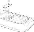
To replace thebackup battery, remove the screw from the backup battery cover, and then remove the cover. Install the new battery, + side up. Replace the cover and secure it with the screw.
Replace the battery compartment cover. Turn the graphing calculator on and adjust the display contrast, if necessary, by pressing [2nd] [up key] or [down key].
Handling a Difficulty
To handle a difficulty, follow these steps.
If you cannot see anything on the screen, you may need to adjust the graphing calculator contrast.
To darken the screen, press and release [2nd], and then press and hold [up key] until the display is sufficiently dark.
To lighten the screen, press and release [2nd], and then press and hold [down key] until the display is sufficiently light.
If an error menu is displayed, follow these steps:
Note the error type (ERR:error type).
Select 2:GOTO, if it is available. The previous screen is displayed with the cursor at or near the error location.
Determine the error.
Correct the expression.
Refer to the Error Conditions table for details about specific errors, if necessary.
If the busy indicator (dotted line) is displayed, a graph or program has been paused; the TI-84 Plus is waiting for input. Press [ENTER] to continue or press [ON] to break.
If a checkerboard cursor is displayed, then either you have entered the maximum number of characters in a prompt, or memory is full. If memory is full:
Press [2nd] [MEM] 2 to display the MEMORY MANAGEMENT / DELETE menu.
Select the type of data you want to delete, or select 1:All for a list of all variables of all types. A screen is displayed listing each variable of the type you selected and the number of bytes each variable is using.
Press [up key] and [down key] to move the selection cursor (â–º) next to the item you want to delete, and then press [DEL].
If the graphing calculator does not seem to work at all, be sure the alkaline batteries are fresh and that they are installed properly.
If the TI-84 Plus does not function even though you are sure that the batteries are fresh, you can try manually resetting it.
Remove all of the AAA batteries from the graphing calculator.
Press and hold the [ON] key for ten seconds.
Replace the batteries.
Turn on the unit.
When you reset your graphing calculator, the contrast sometimes changes. If the screen is faded or blank, adjust the contrast by pressing [2nd] and releasing [up key] or [down key].
If the above solutions do not work you can reset all of the memory. The RAM, user data archive memory, and system variables are restored to factory settings when you reset all memory. All nonsystem variables, applications (Apps), and programs are deleted.
Press [2nd] [MEM] to display the MEMORY menu.
Select 7:Reset to display the RAM ARCHIVE ALL menu.
Press [right key] [right key] to display the ALL menu.
Select 1:All Memory to display the RESET MEMORY menu.
To continue with the reset, select 2:Reset. The message Mem cleared is displayed on the home screen.
Symbols
right arrow dim( (assign dimension) 169 (° (degrees notation) 379
(- (negation) 30, 37, 381
(– (subtraction) 36, 381
(! (factorial) 379
(right arrow Store 20, 375
(right arrow dim( (assign dimension) 155, 358 not equal to 380
square root 36, 381
(blank square, dot, + (pixel mark) 132, 210 plot type, histogram 209
(' (minutes notation) 60, 382 (( ) (parentheses) 29
plot type, normal probability 210 (SigmaInt( (sum of interest) 363 (SigmaPrn( (sum of principal) 368 (* (multiplication) 36, 381
plot type, modified box 209
(integral symbol f(x)dx operation on a graph 90 (*row( 160, 371
(*row+( 371
(+ (addition) 36, 381
(+ (concatenation) 270, 381
(+ (pixel mark) 132, 210 plot type, box 209
(/ (division) 36, 381
(superscript -1 (inverse) 380
(: (colon) 278
(less than) 62, 380
(= (equal-to relational test) 62, 380
(greater than) 62, 380
([ ] (matrix indicator) 148 (^ (power) 36, 380, 381 (less than or equal to) 380
(greater than or equal to) 62, 380 (superscript ² (square) 36, 380
(superscript ³ (cube) 39, 380
cube root 39, 380
(“ †(string indicator) 267
(â–ºDec (to decimal conversion) 39, 357
(â–ºDMS (to degrees/minutes/seconds) 61, 358
(â–ºEff( (to effective interest rate) 261
(â–ºFrac (to fraction) 39, 360
(â–ºNom( (to nominal interest rate) 261, 366
(â–ºPolar (to polar) 56, 368
(â–ºRect (to rectangular) 56, 371
chi-square pdf 244
chi-square test 233, 234, 245 (DeltaTbl (table step variable) 116 (DeltaX window variable 74 (Delta Y window variable 74 (Fcdf( 245
(Fpdf( 245
superscript -1 (inverse) 37
{ } (list indicator) 163
Numerics
10^( (power of ten) 381
1-PropZInt (one-proportion z confidence interval) 232, 369 1-PropZTest (one-proportion z test) 227, 369
Var Stats (one-variable statistics) 200, 377
PropZInt (two-proportion z confidence interval) 232, 369 2-PropZTest (two-proportion z test) 228, 369
2-SampFTest (two-sample F-Test) 235, 372
2-SampTInt (two-sample t confidence interval) 231, 372 2-SampTTest (two-sample t test) 226, 373
2-SampZInt (two-sample z confidence interval) 230, 372 2-SampZTest (two-sample z test) 225, 372
2-Var Stats (two-variable statistics) 200, 377
A
a+bi (rectangular complex mode) 17, 50, 355
about 326
above graph style 71
abs( (absolute value) 46, 55, 152, 354 accuracy information
computational and graphing 398 function limits and results 399 graphing 78
addition (+) 36, 381
alpha cursor 8
alpha-lock 14
alternative hypothesis 219 amortization
Sigma Int( (sum of interest) 363
Sigma Prn( (sum of principal) 368 bal( (amortization balance) 258, 355
calculating schedules 258
formula 389
and (Boolean operator) 63, 354
ANGLE menu 59
angle modes 16
angle( 55, 354 animate graph style 71
ANOVA( (one-way variance analysis) 238, 354, 385
Ans (last answer) 24, 329, 354 APD (Automatic Power Down) 3
applications See examples, applications 36
Apps 20, 328
AppVars 20, 328
arccosine (cos to the -1( ) 36 Archive 21, 330, 354
archive full error 343, 394
garbage collection 340
memory error 340
archived variables 383 arcsine (sin to the -1( ) 36 arctangent (tan to the -1( ) 36 Asm( 294, 354
AsmComp( 294, 354
AsmPrgm( 294, 354
assembly language programs 294 augment( 157, 173, 354 Automatic Power Down (APD) 3 automatic regression equation 196
automatic residual list (RESID) 195 axes format, sequence graphing 107
axes, displaying (AxesOn, AxesOff) 75, 355
AxesOff 75, 355
AxesOn 75, 355
B
backing up calculator memory 348, 351
bal( (amortization balance) 258, 355
batteries 4, 400 below graph style 71 binomcdf( 247, 355
binompdf( 246, 355
block 340
Boolean logic 63
box pixel mark 132, 210 Boxplot plot type 209 busy indicator 8
C
C/Y (compounding-periods-per-year variable) 253, 263 chi square cdf( (chi-square cdf) 355
chi square pdf( (chi-square pdf) 355 chi square-Test (chi-square test) 355 CALCULATE menu 87
Calculate output option 218, 220 cash flow
calculating 257
formula 389
irr( (internal rate of return) 258, 363 npv( (net present value) 258, 367
CATALOG 266
CBL 2â„¢ 293, 346, 361
CBRâ„¢ 293, 346, 361
check memory 326 checkTmr( (check timer) 355 Chi 234
chi-square cdf 245, 355
chi-square goodness of fit test 234 chi-square pdf 244, 355
chi-square test 233, 234, 355
Circle( (draw circle) 128, 355
Clear Entries 326, 356 clearing
all lists (ClrAllLists) 326, 356
drawing (ClrDraw) 123, 356
entries (Clear Entries) 326, 356
home screen (ClrHome) 292, 356
list (ClrList) 194, 356
table (ClrTable) 292, 356
Clock 9
Clock Off 11
Clock On 10
ClockOff, turn clock off 356 ClockOn, turn clock on 356 ClrAllLists (clear all lists) 326, 356
ClrDraw (clear drawing) 123, 356
ClrHome (clear home screen) 292, 356
ClrList (clear list) 194, 356
ClrTable (clear table) 292, 356 coefficients of determination (r2, R2) 196 colon separator (:) 278
combinations (nCr) 57, 366
compiling an assembly program 294, 354 complex
modes (a+bi, re^thetai) 17, 50, 355, 370
numbers 17, 50, 370
compounding-periods-per-year variable (C/Y) 253, 263
concatenation (+) 270, 381
confidence intervals 36, 220
conj( (conjugate) 54, 356
Connected (plotting mode) 17, 356
connecting two calculators 346, 349
contrast (display) 4
convergence, sequence graphing 110 conversions
â–ºDec (to decimal) 39, 357
â–ºDMS (to degrees/minutes/ seconds) 61, 358
â–ºEff (to effective interest rate) 261
4F3 4D 50
â–ºFrac (to fraction conversion) 39, 360
4n/d3 4Un/d 49
â–ºNom (to nominal interest rate conversion) 261, 366
â–ºPolar (to polar conversion) 56, 368
â–ºRect (to rectangular conversion) 56, 371
Equâ–ºString( (equation-to-string conversion) 270, 359
Listâ–ºmatr( (list-to-matrix conversion) 158, 173, 364
Matrâ–ºlist( (matrix-to-list conversion) 157, 174, 365
Pâ–ºRx(, Pâ–ºRy( (polar-to-rectangular conversion) 61,
3d69
Râ–ºPr(, Râ–ºPtheta( (rectangular-to-polar conversion) 372
Râ–ºPr(, Râ–ºPtheta( (rectangular-to-polar conversion) 61
Stringâ–ºEqu( (string-to-equation conversion) 271, 375 convert time, timeCnv( ) 376
CoordOff 75, 356
CoordOn 75, 356
correlation coefficient (r) 196 cos( (cosine) 36, 356
cos superscript -1( (arccosine) 36, 356
cosh( (hyperbolic cosine) 273, 356
cosh superscript -1( (hyperbolic arccosine) 273, 356 cosine (cos( ) 36
cosine (cos( ) 356
cross pixel mark (+) 132, 210
cube (³) 39, 380
cube root 39
cube root 380
cubic regression (CubicReg) 201, 356
CubicReg (cubic regression) 201, 356
cumSum( (cumulative sum) 158, 170, 357
cumulative sum (cumSum( ) 158, 170 cumulative sum (cumSum( ) 357 cursors 8, 14
D
Data input option 218, 219 dayOfWk( (day of week) 357 days between dates (dbd( ) 261
days between dates (dbd( ) 357, 390 dbd( (days between dates) 261, 357, 390 decimal mode (float or fixed) 16
decrement and skip (DS< less than( ) 286 decrement and skip (DS< less than( ) 358 definite integral 40, 89, 96
defragmenting 340
Degree angle mode 16, 60, 357
degrees notation 60, 379
delete variable contents (DelVar) 287, 357 deleting items from memory 329 DependAsk 116, 118, 357
DependAuto 116, 118, 357
derivative See numerical derivative 36 det( (determinant) 155, 357 determinant (det( ) 155
determinant (det( ) 357 DiagnosticOff 196, 357
DiagnosticOn 196, 357
diagnostics display mode(r, r2, R2) 196 differentiation 42, 89, 96, 101
dim( (dimension) 155, 169, 357
dimensioning a list or matrix 155, 169, 357
Disp (display) 290, 358
DispGraph (display graph) 291, 358
display contrast 4
display cursors 8
Displaying the Clock Settings 9 DispTable (display table) 291, 358 DISTR (distributions menu) 241
DISTR DRAW (distributions drawing menu) 248 distribution functions
binomcdf( 247, 355
binompdf( 246, 355 chi square cdf( 355 chi square ²pdf( 355 Fcdf( 244, 375
Fpdf( 243, 376
geometcdf( 248, 361
geometpdf( 248, 361
invNorm( 243, 363
normalcdf( 242, 366
normalpdf( 242, 366
poissoncdf( 247, 368
poissonpdf( 247, 368 distribution shading instructions
Shade_t( 249, 374
Shadechi²( 250, 374
ShadeF( 250, 374
ShadeNorm( 249, 374
division (/) 36, 381
Delta List( 171, 364
DMS (degrees/minutes/seconds entry notation) 60, 382
Dot (plotting mode) 17, 358 dot graph style 71
dot pixel mark (•) 132, 210
dr/d theta operation on a graph 101 DRAW menu 122
Draw output option 218, 220 DRAW POINTS menu 131
DRAW STO (draw store menu) 134 DrawF (draw a function) 127, 358 drawing on a graph
circles (Circle( ) 128
functions and inverses (DrawF, DrawInv) 127 line segments (Line( ) 124
lines (Horizontal, Line(, Vertical) 125 points (Pt-Change, Pt-Off, Pt-On) 131 tangents (Tangent) 126
text (Text) 129
using Pen 130
DrawInv (draw inverse) 127, 358
DS< less than( (decrement and skip) 286, 358 DuplicateName menu 350
dx/dt operation on a graph 89, 96 dy/dx operation on a graph 89, 96, 101
E
E (exponent) 12, 15, 358
e^( (exponential) 37, 358 edit keys table 13
Else 282
End 283, 359
Eng (engineering notation mode) 15, 359 ENTRY (last entry key) 22
entry cursor 8
EOS (Equation Operating System) 29 eqn (equation variable) 42
Equâ–ºString( (equation-to-string conversion) 270, 359
equal-to relational test (=) 62, 380 Equation Operating System (EOS) 29 Equation Solver 42
equations with multiple roots 44 errors
diagnosing and correcting 33 messages 394
examples—applications area between curves 316
areas of regular n-sided polygons 321 box plots 306
box with lid 299
defining a 299
defining a table of values 300 setting the viewing window 302 tracing the graph 303
zooming in on the graph 304 zooming in on the table 301
cobweb attractors 312
fundamental theorem of calculus 319 guess the coefficients 313 inequalities 309
mortgage payments 323
parametric equations, ferris wheel problem 317 piecewise functions 308
quadratic formula
converting to a fraction 297 displaying complex results 298 entering a calculation 297
Sierpinski triangle 311
solving a system of nonlinear equations 310 unit circle and trig curves 315
examples—Getting Started coin flip 35
compound interest 253 drawing a tangent line 121 financing a car 252
forest and trees 102 generating a sequence 161
mean height of a population 215 path of a ball 91
pendulum lengths and periods 178 polar rose 97
roots of a function 115 sending variables 344
solving a system of linear equations 144 unit circle 137
volume of a cylinder 275 examples—miscellaneous
calculating outstanding loan balances 259 convergence 110
daylight hours in Alaska 204 predator-prey model 111
examplesóGetting Started graphing a circle 65
exponential regression (ExpReg) 202, 359
expr( (string-to-expression conversion) 270, 359
ExpReg (exponential regression) 202, 359
expression 11
converting from string (expr( ) 270 converting from string (expr( ) 359 turning on and off (ExprOn 76, 359
ExprOff (expression off) 76, 359
ExprOn (expression on) 76, 359
F
Faceplates 8
factorial (!) 379 family of curves 77 Fill( 156, 359
FINANCE CALC menu 254 FINANCE VARS menu 262
financial functions amortization schedules 258
cash flows 257
days between dates 261 interest rate conversions 261 payment method 262
time value of money (TVM) 255 Fix (fixed-decimal mode) 16, 359
fixed-decimal mode (Fix) 16, 359
Float (floating-decimal mode) 16, 359
floating-decimal mode (Float) 16, 359 fMax( (function maximum) 360 fMin( (function minimum) 40, 360
fnInt( (function integral) 41, 360
FnOff (function off) 70, 360
FnOn (function on) 70, 360
For( 283, 360
format settings 74, 107 formulas
amortization 389
ANOVA 385
cash flow 389
days between dates 390 interest rate conversions 390 logistic regression 384
sine regression 384
time value of money 387 two-sample F-Test 385 two-sample t test 386
fPart( (fractional part) 47, 154, 360 fractions
n/d 18, 50
Un/d 18, 50
free-moving cursor 78
frequency 199
Full (full-screen mode) 17, 360
full-screen mode (Full) 17, 360
Func (function graphing mode) 16, 360 function graphing
accuracy 78
CALC (calculate menu) 87 defining and displaying 66 defining in the Y= editor 68
defining on the home screen, in a program 68 deselecting 69
displaying 66, 73, 76
Delta X and Delta Y window variables 74 evaluating 69
family of curves 77 format settings 74
free-moving cursor 78
graph styles 71 maximum of (fMax( ) 40
maximum of (fMax( ) 360 minimum of (fMin( ) 360 modes 16, 67, 360
moving the cursor to a value 79 overlaying functions on a graph 77 panning 80
pausing or stopping a graph 76 Quick Zoom 80
selecting 69, 70, 360
shading 72
Smart Graph 76
tracing 78
viewing window 73
window variables 73
Y= editor 68
ZOOM MEMORY menu 85
ZOOM menu 80 function integral (fnInt( ) 41 function integral (fnInt( ) 360 function, definition of 12
functions and instructions table 354 future value 253, 257
FV (future-value variable) 253, 263
G
garbage collecting 339
GarbageCollect 341, 360
gcd( (greatest common divisor) 48, 360 GDB (graph database) 135
geometcdf( 248, 361
geometpdf( 248, 361
Get( (get data from CBL 2â„¢ or CBRâ„¢) 293, 361 GetCalc( (get data from TI-84 Plus) 292, 361 getDate, get current date 361
getDtFmt, get date format 361 getDtStr( (get date string) 361 getKey 292, 361
getTime, get current time 361
Getting Started See examples, Getting Started 36 getTmFmt, get time format 361
getTmStr( (get time string) 361 Goto 285, 361
graph database (GDB) 135 graph style
above 71
animate 71
below 71
dot 71
line 71
path 71
shade above 71
shade below 71
thick 71
graph styles 71
graphing modes 16
graphing-order modes 17
GraphStyle( 288, 362
graph-table split-screen mode (G-T) 17, 140, 362
greater than (>) 62, 380
greater than or equal to 62, 380 greatest common divisor (gcd( ) 48 greatest common divisor (gcd( ) 360 greatest integer (int( ) 47, 154 greatest integer (int( ) 363
GridOff 75, 362
GridOn 75, 362
grouping 336
G-T (graph-table split-screen mode) 17, 140, 362
H
Histogram plot type 209 home screen 5
scrolling 5, 22
Horiz (horizontal split-screen mode) 17, 139, 362
Horizontal (draw line) 125, 362
hyperbolic functions 273
hypothesis tests 223
I
i (complex number constant) 52
I% (annual interest rate variable) 253, 263 identity( 156, 362
If instructions
If 282, 362
If-Then 282, 362
If-Then-Else 282, 362
imag( (imaginary part) 55, 362 imaginary part (imag( ) 55 imaginary part (imag( ) 362 implied multiplication 29
increment and skip (IS> greater than( ) 286 increment and skip (IS> greater than ( ) 363 independent variable 116, 118, 362
IndpntAsk 116, 118, 362
IndpntAuto 116, 118, 362 inferential stat editors 218 inferential statistics
alternative hypotheses 219
bypassing editors 220
calculating test results (Calculate) 220 confidence interval calculations 220 data input or stats input 219
entering argument values 219 graphing test results (Draw) 220 input descriptions table 239 pooled option 220
STAT TESTS menu 221
test and interval output variables 240 inferential statistics See stat tests 36 Input 289, 362
insert cursor 8
Installing New Faceplates 9 Installing new faceplates 9 inString( (in string) 271, 363 instruction, definition of 13
int( (greatest integer) 47, 154, 363
integer part (iPart( ) 47, 154 integer part (iPart( ) 363
integral See numerical integral 36
interest rate conversions
â–ºEff( (compute effective interest rate) 261
â–ºNom( (compute nominal interest rate) 261
calculating 261
formula 390
internal rate of return (irr( ) 258 internal rate of return (irr( ) 363 intersect operation on a graph 89 inverse (superscript -1) 37, 380
inverse cumulative normal distribution (invNorm( ) 243 inverse cumulative normal distribution (invNorm( ) 363 inverse trig functions 36
invNorm( (inverse cumulative normal distribution) 243, 363 invT (inverse Student T distribution) 243
iPart( (integer part) 47, 154, 363 irr( (internal rate of return) 258, 363
IS> greater than ( (increment and skip) 286, 363 isClockOn, is clock on 363
K
keyboard
layout 1
math operations 36
key-code diagram 292
L
L (user-created list name symbol) 174 LabelOff 76, 363
LabelOn 76, 363 labels
graph 76, 363
program 285, 363
Last Entry 22
Lbl (label) 285, 363
lcm( (least common multiple) 48, 364 least common multiple (lcm( ) 48 least common multiple (lcm( ) 364 length( of string 271, 364
less than (<) 62, 380
less than or equal to 62, 380 line graph style 71
line segments, drawing 124 Line( (draw line) 125, 364
lines, drawing 125
LINK RECEIVE menu 350 LINK SEND menu 347
linking
receiving items 350
to a CBL 2â„¢ or CBRâ„¢ 346 to a PC or Macintosh 346
to a TI-84 Plus Silver Edition or TI-84 Plus 351 transmitting items 344
two TI-84 Plus units 348
Link-Receive L1 (or any file) to Restore message 392 LinReg(a+bx) (linear regression) 202, 364
LinReg(ax+b) (linear regression) 201, 364 LinRegTTest (linear regression t test) 236, 364 LinReqTInt (confidence interval for slope) 237 LIST MATH menu 175
LIST NAMES menu 164 LIST OPS menu 168
Listâ–ºmatr( (lists-to-matrix conversion) 158, 173, 364
lists
accessing an element 164 attaching formulas 165, 166, 188 clearing all elements 187 copying 163
creating 162, 186
deleting from memory 164, 329
detaching formulas 166, 190
dimension 163
entering list names 165, 185 indicator ({ }) 163
naming lists 162
storing and displaying 163
using to graph a family of curves 77, 164 using with math operations 36, 167
ln( 37, 364
LnReg (logarithmic regression) 202, 364
log( 37, 364
Logistic (regression) 203, 364 logistic regression formula 384
M
Manual Linear Fit 198, 205 marked for deletion 340
MATH CPX (complex menu) 54 MATH menu 38
MATH NUM (number menu) 45 math operations 36
MATH PRB (probability menu) 56
Matrâ–ºlist( (matrix-to-list conversion) 157, 174, 365 matrices
accessing elements 150
copying 150
defined 145
deleting from memory 146 dimensions 146, 155, 156 displaying a matrix 149 displaying matrix elements 146 editing matrix elements 147 indicator ([ ]) 148
math functions 151
matrix math functions (det(, superscript T, dim(, Fill(, identity(, randM(, augment(, Matrâ–ºlist(,
Listâ–ºmatr(, cumSum( ) 154 quick matrix 143
relational operations 153
row operations (ref(, rref(, rowSwap(, row+(, *row(,
*row+( ) 158
selecting 145
viewing 146 MATRX EDIT menu 145
MATRX MATH menu 154
max( (maximum) 48, 175, 365 maximum of a function (fMax( ) 40 maximum of a function (fMax( ) 360 maximum operation on a graph 88 mean( 175, 365
Med(Med (median-median) 200
median( 175, 365
Med-Med (median-median) 365 Mem Mgmt/Del menu 327 memory
backing up 351
checking available 326
clearing all list elements from 330 clearing entries from 329
deleting items from 329 error 341
insufficient during transmission 353 resetting defaults 334
resetting memory 334
MEMORY menu 326
Menu( (define menu) 286, 365
menus 25, 26
defining (Menu( ) 286 defining (Menu( ) 365 scrolling 26
shortcut 1, 6
min( (minimum) 48, 175, 365 minimum of a function (fMin( ) 40 minimum of a function (fMin( ) 360 minimum operation on a graph 88 minutes notation (') 60, 382 ModBoxplot plot type 209
mode
Answers 18
Classic 5, 18
MathPrint 5, 18
mode settings 14
a+bi (complex rectangular) 17, 50, 355
Connected (plotting) 17, 356
Degree (angle) 16, 61, 357
Dot (plotting) 17, 358
Eng (notation) 15, 359
Fix (decimal) 16, 359
Float (decimal) 16, 359
Full (screen) 17, 360
Func (graphing) 16, 360
G-T (screen) 17, 362
Horiz (screen) 17, 362
Normal (notation) 15, 366
Par/Param (graphing) 16, 367
Pol/Polar (graphing) 16, 368
Radian (angle) 16, 61, 370 re^theta i (complex polar) 370 re^theta i (complex polar) 17, 50
Real 17, 370
Sci (notation) 15, 373
Seq (graphing) 16, 373
Sequential (graphing order) 17, 373
Simul (graphing order) 17, 374 modified box plot type 209 multiple entries on a line 12 multiplication (*) 36, 381
multiplicative inverse 37
N
N (number of payment periods variable) 253, 263 n/d 18, 50
nCr (number of combinations) 57, 366
nDeriv( (numerical derivative) 40, 366
negation (-) 30, 37, 381
nonrecursive sequences 105
normal distribution probability (normalcdf( ) 242, 366 Normal notation mode 15, 366
normal probability plot type 210
normalcdf( (normal distribution probability) 242 normalpdf( (probability density function) 242, 366 NormProbPlot plot type 210
not equal to 62, 380
not( (Boolean operator) 63, 367
nPr (permutations) 57, 367
npv( (net present value) 258, 367
numerical derivative 40, 89, 96, 101
numerical integral 40, 90
O
Omit 338, 351
one-proportion z confidence interval (1-PropZInt) 232, 369 one-proportion z test (1-PropZTest) 227, 369
one-sample t confidence interval (TInterval) 229, 376 one-variable statistics (1-Var Stats) 200, 377
or (Boolean) operator 63, 367 order of evaluating equations 29 Output( 142, 291, 367
Overwrite 338, 350
Overwrite All 338
P
P/Y (number-of-payment-periods-per-year variable) 253, 263
Pâ–ºRx(, Pâ–ºRy( (polar-to-rectangular conversions) 61, 369
panning 80
Par/Param (parametric graphing mode) 16, 367
parametric equations 94 parametric graphing
CALC (calculate operations on a graph) 96 defining and editing 94
free-moving cursor 95
graph format 94
graph styles 93
moving the cursor to a value 96 selecting and deselecting 94 setting parametric mode 93 tracing 96
window variables 94
Y= editor 93
zoom operations 96
parentheses 29 path graph style 71 Pause 284, 367 pausing a graph 76 Pen 130
permutations (nPr) 57, 367
phase plots 111
Pic (pictures) 134
pictures (Pic) 134
pixels in Horiz/G-T modes 133, 141
Plot1( 210, 367
Plot2( 210, 367
Plot3( 210, 367
PlotsOff 212, 368
PlotsOn 212, 368
plotting modes 17 plotting stat data 208
PMT (payment amount variable) 253, 263
Pmt_Bgn (payment beginning variable) 262, 368
Pmt_End (payment end variable) 262, 368
poissoncdf( 247, 368
poissonpdf( 247, 368
Pol/Polar (polar graphing mode) 16, 98, 368
polar equations 98
polar form, complex numbers 52 polar graphing
CALC (calculate operations on a graph) 101 defining and displaying 98
equations 98
free-moving cursor 100
graph format 99
graph styles 98
mode (Pol/Polar) 16, 98, 368 moving the cursor to a value 100 selecting and deselecting 98 tracing 100
window variables 99
Y= editor 98
ZOOM operations 101
PolarGC (polar graphing coordinates) 75, 368
pooled option 218, 220
power (^) 36, 380, 381 power of ten (10^( ) 37 power of ten (10^( ) 381 present value 253, 256
previous entry (Last Entry) 22 prgm (program name) 287, 368
PRGM CTL (program control menu) 281 PRGM EDIT menu 280
PRGM EXEC menu 280 PRGM NEW menu 277
probability 56
probability density function (normalpdf( ) 242 probability density function (normalpdf( ) 366 prod( (product) 176, 368
programming
copying and renaming 280 creating new 277
defined 276
deleting 277
deleting command lines 280 editing 279
entering command lines 278 executing 279
inserting command lines 280 instructions 281
name (prgm) 287, 368
renaming 280
running assembly language program 294 stopping 279
subroutines 293
Prompt 290, 369
Pt-Change( 132, 369
Pt-Off( 132, 369
Pt-On( 131, 369
PV (present value variable) 253, 263
p-value 240
PwrReg (power regression) 203, 369
Pxl-Change( 133, 369
Pxl-Off( 133, 369
Pxl-On( 133, 369
pxl-Test( 133, 369
Q
QuadReg (quadratic regression) 201, 370
QuartReg (quartic regression) 202, 370
Quick Zoom 80
Quit 338, 351
R
r (correlation coefficient) 196
R (radian notation) 61, 379
r2, R2 (coefficients of determination) 196
Râ–ºPr(, Râ–ºP theta( (rectangular-to-polar conversions) 372 Râ–ºPr(, Râ–ºP theta( (rectangular-to-polar conversions) 61 Radian angle mode 16, 61, 370
radian notation (superscript r) 61, 379 RAM ARCHIVE ALL menu 333
rand (random number) 57, 370
randBin( (random binomial) 59, 370
randInt( (random integer) 58, 370
randIntNoRep( 59
randM( (random matrix) 157, 370
randNorm( (random Normal) 58, 370
random seed 57
RCL (recall) 21
re^theta i (polar complex mode) 370 re^theta i (polar complex mode) 17, 50 Real mode 17, 370
real( (real part) 54, 370
RecallGDB 136, 370
RecallPic 135, 370
rectangular form, complex numbers 52
RectGC (rectangular graphing coordinates) 75, 371
recursive sequences 105
re-enabling a disabled calculator 392 ref( (row-echelon form) 159, 371
RegEQ (regression equation variable) 196, 329 regression model
automatic regression equation 196 automatic residual list feature 195 diagnostics display mode 196 models 200
relational operations 62, 153
remainder( 49 Removing a Faceplate 9 Repeat 284, 371
RESET MEMORY menu 336
resetting
all memory 336
archive memory 335
defaults 334
memory 334
RAM memory 334 residual list (RESID) 195 Return 287, 371
root (xth root) 40, 379 root of a function 88 round( 47, 152, 371
row+( 371
rowSwap( 159, 371
rref( (reduced-row-echelon form) 159, 372
S
Sci (scientific notation mode) 15, 373
scientific notation 12
screen modes 17 second cursor (2nd) 8 second key (2nd) 2
seconds DMS notation (â€) 60 sector 340
Select( 171, 373 selecting
data points from a plot 172
functions from the home screen or a program 70 functions in the Y= editor 70
stat plots from the Y= editor 70
Send( (send to CBL 2â„¢ or CBRâ„¢) 293, 373 SendID 347
sending See transmitting 36
SendSW 347
Seq (sequence graphing mode) 16, 373
seq( (sequence) 170, 373 sequence graphing
axes format 107
CALC (calculate menu) 108 evaluating 109
free-moving cursor 107
graph format 107
graph styles 104
moving the cursor to a value 108 nonrecursive sequences 105
recursive sequences 105 selecting and deselecting 104
TI-84 Plus versus TI-82 table 114 tracing 108
web plots 109
window variables 106
Y= editor 103
ZOOM (zoom menu) 108
Sequential (graphing order mode) 17, 373 setDate( (set date) 373
setDtFmt( (set date format) 373 setTime( (set time) 373
setting
display contrast 4
graph styles 71
graph styles from a program 72 modes 15
modes from a program 15 split-screen modes 138
split-screen modes from a program 142 tables from a program 116
setTmFmt( (set time format) 373 SetUpEditor 194, 373
shade above graph style 71 shade below graph style 71 Shade( 128, 373
Shade_t( 249, 374
Shade chi square( 250, 374
ShadeF( 250, 374
ShadeNorm( 249, 374
shading graph areas 72, 128
Simul (simultaneous graphing order mode) 17, 374 sin( (sine) 36, 374
sin superscript -1( (arcsine) 36, 374
sine (sin( ) 36
sine (sin( ) 374
sinh( (hyperbolic sine) 273, 374
sinh superscript -1( (hyperbolic arcsine) 273, 374
SinReg (sinusoidal regression) 203, 374
Smart Graph 76
solve( 44, 374
Solver 42
solving for variables in the equation solver 43 SortA( (sort ascending) 168, 194, 374
SortD( (sort descending) 168, 194, 374 split-screen modes
G-T (graph-table) mode 140 Horiz (horizontal) mode 139 setting 138, 142
split-screen values 130, 133, 141
square (superscript ²) 36, 380
square root 36
square root 381 startTmr, start timer 374 STAT CALC
Stat Wizards 198 STAT CALC menu 198 STAT EDIT menu 193
stat list editor
attaching formulas to list names 188 clearing elements from lists 187 creating list names 186
detaching formulas from list names 190 displaying 184
edit-elements context 192
editing elements of formula-generated lists 190 editing list elements 187
entering list names 185 enter-names context 193
formula-generated list names 189 removing lists 186
restoring list names L1–L6 186 switching contexts 190
view-elements context 192
view-names context 193 STAT PLOTS menu 210
stat tests and confidence intervals
PropZInt (one-proportion z confidence interval) 232 1-PropZTest (one-proportion z test) 227
PropZInt (two-proportion z confidence interval) 232 2-PropZTest (two-proportion z test) 228
2-SampFTest (two-sample F-Test) 235
2-SampTInt (two-sample t confidence interval) 231 2-SampTTest (two-sample t test) 226
2-SampZInt (two-sample z confidence interval) 230 2-SampZTest (two-sample z test) 225
ANOVA( (one-way analysis of variance) 236 chi-square test 233, 234
chi-square test 233, 234
LinRegTTest (linear regression t test) 236 TInterval (one-sample t confidence interval) 229 T-Test (one-sample t test) 224
ZInterval (one-sample z confidence interval) 229 Z-Test (one-sample z test) 223
STAT TESTS menu 221 STAT WIZARDS 1, 198, 199
statistical distribution functions See distribution functions 36
statistical plotting 208
Boxplot (regular box plot) 209 defining 210
from a program 212 Histogram 209
ModBoxplot (modified box plot) 209 NormProbPlot (normal probability plot) 210 tracing 212
turning on/off stat plots 70, 212
viewing window 212
xyLine 208
statistical variables table 206 Stats input option 218, 219
stdDev( (standard deviation) 176, 375
Stop 287, 375
Store (right arrow) 20, 375
StoreGDB 135, 375
StorePic 134, 375 storing
graph databases (GDBs) 135 graph pictures 134
variable values 20
Stringâ–ºEqu( (string-to-equation conversions) 271, 375 strings
concatenation (+) 270, 381
converting 270
defined 267
displaying contents 269
entering 267
functions in CATALOG 269 indicator (â€) 267
length (length( ) 271 length (length( ) 364 storing 268
variables 268 student-t distribution
probability (tcdf( ) 244
probability (tcdf( ) 375 student-t distribution
probability density function (tpdf( ) 243 probability density function (tpdf( ) 376
sub( (substring) 272, 375
subroutines 287
subtraction (–) 36, 381
sum( (summation) 176, 375
system variables 383
T
superscript T (transpose matrix) 155, 379 TABLE SETUP screen 116
tables
description 118
variables 116, 117
tan( (tangent) 36, 375
tan superscript -1 ( (arctangent) 36, 375
tangent (tan( ) 36 tangent (tan( ) 375
tangent lines, drawing 126 Tangent( (draw line) 126, 375
tanh( (hyperbolic tangent) 273, 375
tanh superscript -1( (hyperbolic arctangent) 273, 375 TblStart (table start variable) 116
tcdf( (student-t distribution probability) 244, 375 TEST (relational menu) 62
TEST LOGIC (Boolean menu) 63 Text(
instruction 129, 142, 376
placing on a graph 129, 142
Then 282, 362
thick graph style 71 TI Connectâ„¢ 346 TI-84 Plus
key code diagram 292 keyboard 1
Time axes format 107, 376 time value of money (TVM)
C/Y variable (number of compounding periods per year) 263
calculating 255
formulas 387
FV variable (future value) 263
I% variable (annual interest rate) 263
N variable (number of payment periods) 263
P/Y variable (number of payment periods per year) 263 PMT variable (payment amount) 263
PV variable (present value) 263 TVM Solver 253
tvm_FV (future value) 257, 376 tvm_I% (interest rate) 376 tvm_I% (interest rate) 256
tvm_N (# payment periods) 256, 376
tvm_Pmt (payment amount) 256, 376
tvm_PV (present value) 256, 376
variables 262
timeCnv( ), convert time 376
TInterval (one-sample t confidence interval) 376 TInterval (one-sample t confidence interval) 229
tpdf( (student-t distribution probability density function) 243, 376
TRACE
cursor 79
entering numbers during 79, 96, 100, 108
expression display 76, 79
Trace instruction in a program 80, 376 transmitting
error conditions 352 from a TI-83 351
from a TI-83 Plus Silver Edition or TI-83 Plus 351 from a TI-84 Plus Silver Edition or TI-84 Plus 351 stopping 348
to a TI-84 Plus Silver Edition or TI-84 Plus 348 transpose matrix (superscript T) 155, 379
trigonometric functions 36
T-Test (one-sample t test) 224, 376
turn clock off, ClockOff 356 turn clock on, ClockOn 356 turning on and off
axes 75
calculator 3
coordinates 75
expressions 76
functions 70
grid 75
labels 76
points 131
stat plots 70, 212
tvm_FV (future value) 257, 376 tvm_I% (interest rate) 376 tvm_I% (interest rate) 256
tvm_N (# payment periods) 256, 376
tvm_Pmt (payment amount) 256, 376
tvm_PV (present value) 256, 376
two-proportion z confidence interval (2-PropZInt) 232, 369 two-proportion z test (2-PropZTest) 228, 369
two-sample F-Test formula 385
two-sample t test formula 386
two-variable statistics (2-Var Stats) 200, 377
U
u sequence function 103 Un/d 18, 50
UnArchive 21, 330, 377
ungrouping 336
user variables 383
uv/uvAxes (axes format) 107, 377
uw/uwAxes (axes format) 107, 377
V
v sequence function 103 value operation on a graph 87 variables
complex 19
displaying and storing values 21 equation solver 43
graph databases 19
graph pictures 19
independent/dependent 118
list 19, 162
matrix 19, 145
real 19
recalling values 21
solver editor 43
statistical 206
string 268
test and interval output 240 types 19
user and system 20, 383 VARS and Y-VARS menus 27
variance of a list (variance( ) 176 variance of a list (variance( ) 377 variance( (variance of a list) 176, 377 VARS menu
GDB 27
Picture 27
Statistics 27
String 27
Table 27
Window 27
Zoom 27
Vertical (draw line) 125, 377
viewing window 73
vw/uvAxes (axes format) 107, 377
W
w sequence function 103 Web (axes format) 107, 377
web plots 109
While 283, 377 window variables
function graphing 73
parametric graphing 95
polar graphing 99
X
x (root) 379
XFact zoom factor 86 x-intercept of a root 88
xor (Boolean) exclusive or operator 63, 377 xth root 40
xyLine plot type 208
Y
Y= editor
function graphing 68
parametric graphing 93
polar graphing 98
sequence graphing 103 YFact zoom factor 86
Y-VARS menu Function 28
On/Off 28
Parametric 28
Polar 28
Z
ZBox 81, 377
ZDecimal 82, 377
zero operation on a graph 88 ZInteger 83, 378
ZInterval (one-sample z confidence interval) 229, 378 zoom 80, 81, 82, 83, 85, 86
cursor 81
factors 86
function graphing 80
parametric graphing 96
polar graphing 101
sequence graphing 108
Zoom In (zoom in) 82, 378 ZOOM MEMORY menu 85
ZOOM menu 80
Zoom Out (zoom out) 82, 378 ZoomFit (zoom to fit function) 83, 378
ZoomRcl (recall stored window) 86, 378
ZoomStat (statistics zoom) 83, 378
ZoomSto (store zoom window) 85, 378 ZPrevious (use previous window) 379 ZSquare (set square pixels) 82, 379
ZStandard (use standard window) 83, 379
Z-Test (one-sample z test) 223, 379
ZTrig (trigonometric window) 83, 379
|
32 |
right arrow |
scat- ter plot
(shad ed cell: see note below ) |
shade d rect- angle |
solid rect- angle |
blank rect- angle |
histo- gram
(shad ed cell: see note below ) |
space
(shad ed cell: see note below ) |
xyLin e |
Norm Prob- Plot |
Mod- Box- Plot |
Box- plot |
[STA T PLO T] |
[TBL SET] |
[FOR MAT] |
[CAL C] |
47 |
|
|
48 |
[TAB LE] |
greate r than |
much greate r than |
greate r than abso- lute value |
[QUI T] |
[INS] |
[A- LOC K] |
[LIN K] |
[LIST ] |
[TES T] |
[AN GLE] |
[DRA W]
(shad ed cell: see note below ) |
[DIS TR] |
[MAT RIX]
(shad ed cell: see note below ) |
[SIN super -1] |
63 |
|
|
64 |
[COS super -1] |
[TAN super -1] |
[pi] |
[squa re root] |
[EE] |
[{] |
[}] |
[10 super x] |
[ [ ] |
[ ] ] |
[e super x] |
[RCL ] |
[ME M] |
[OFF ] |
[CAT ALO G] |
[spac e key] |
79 |
|
80 |
Prod- uct (capi- tal Pi) |
[MAT RX] |
Sigm a |
[FIN ANC E] |
[i] |
page icon |
[ANS ] |
[ENT RY] |
[SOL VE] |
[F1] |
[F2] |
95 |
|
96 |
[F3] |
[F4] |
[F5] |
[L1] |
[L2] |
[L3] |
[L4] |
[L5] |
[L6] |
[ - ] |
[(-)] |
page icon with capi- tal P |
[Y=] |
111 |
|||
|
112 |
[WIN DOW ] |
[ZOO M] |
[TRA CE] |
[GRA PH] |
[ALP HA] |
[CLE AR] |
[STO right arrow ] |
[2nd] |
[MO DE] |
[DEL ] |
[left key] |
[up key] |
[right key] |
127 |
|||
|
128 |
[ALP HA] |
[X, T, theta, n] |
[STA T] |
[dow n key] |
[APP S] |
[MAT H] |
[MAT RX] |
[PRG M] |
143 |
||||||||
|
144 |
[VAR S] |
[CLE AR] |
[x super -1] |
[SIN] |
[COS ] |
[TAN ] |
[car- et] |
[x super -1] |
159 |
||||||||
|
160 |
[x super 2] |
[,] |
[ ( ] |
[ ) ] |
[divi- sion key] |
¶ |
[LOG ] |
[7] |
[8] |
[9] |
[mul- tipli- cation key] |
175 |
|||||
|
176 |
[TRI GGE R] |
[ON/ HAL T] |
[LN] |
[4] |
[5] |
[6] |
[ - ] |
[STO right arrow ] |
191 |
||||||||
|
192 |
[1] |
[2] |
[3] |
[+] |
p-hat |
[ON] |
[0] |
[.] |
[(-)] |
[ENT ER] |
207 |
||||||
|
208 |
histo- gram |
xyLin e |
Norm Prob- Plot |
Mod- Box- Plot |
Box- plot |
i |
re- verse A |
L |
N |
F |
F (bold) |
re- verse up arrow |
down and to left arrow |
223 |
|||
|
224 |
E |
" |
* |
E (bold) |
I% |
line |
thick |
above |
below |
path |
ani- mate |
dot |
[CON T] |
239 |
|
240 |
direc- tional keys icon |
[Y- VAR S] |
[n] |
[U sub n - 1] |
[V sub n - 1] |
p-hat |
mean of x |
mean of y |
mean of x |
mean of y |
255 |
Note: The symbols in shaded cells have been assigned SpecialKeySymbol conditional tag. The tag will be included when you paste the symbol into your document, and it is required for correct output by WebWorks Publisher.